Testing Predictions of the Programmed and Stochastic Theories of Aging: Comparison of Variation in Age at Death, Menopause, and Sexual Maturation
N. S. Gavrilova1*, L. A. Gavrilov1, F. F. Severin2, and V. P. Skulachev2
1Center on Aging, NORC at The University of Chicago, 1155 East 60th str., Chicago, IL 60637, USA; fax: 1-773-643-8608; E-mail: nsgavril@alumni.uchicago.edu2Belozersky Institute of Physico-Chemical Biology and Institute of Mitoengineering, Lomonosov Moscow State University, 119991 Moscow, Russia
* To whom correspondence should be addressed.
Received March 27, 2012
One of the arguments against aging being programmed is the assumption that variation in the timing of aging-related outcomes is much higher compared to variation in timing of the events programmed by ontogenesis. The main objective of this study was to test the validity of this argument. To this aim, we compared absolute variability (standard deviation) and relative variability (coefficient of variation) for parameters that are known to be determined by the developmental program (age at sexual maturity) with variability of characteristics related to aging (ages at menopause and death). We used information on the ages at sexual maturation (menarche) and menopause from the nationally representative survey of the adult population of the United States (MIDUS) as well as published data for 14 countries. We found that coefficients of variation are in the range of 8-13% for age at menarche, 7-11% for age at menopause, and 16-21% for age at death. Thus, the relative variability for the age at death is only twice higher than for the age at menarche, while the relative variability for the age at menopause is almost the same as for the age at menarche.
KEY WORDS: aging, variability, menarche, menopause, lifespanDOI: 10.1134/S0006297912070085
The question of whether or not aging is programmed is currently being debated by gerontologists [1, 2]. Many researchers believe that there is no special genetic program of aging [1, 3-6], while others recognize the possibility of both programmatic and non-programmatic components of aging [2, 7]. Recently, more researchers have begun to consider aging as a programmed process [8-24]. In this work we tested the validity of one of the arguments used by the opponents of programmed aging, i.e. that variation in individual lifespans and other aging-related outcomes (like age at menopause) is too high compared to variation of events related to the ontogenesis program [25]. We found that relative variability of (i) ages when such an ontogenesis program-controlled event as sexual maturity in women happens and (ii) aging-related events (ages of menopause and death) are, in fact, of the same order of magnitude. Thus, parameters of human ontogenesis and senescence have similar relative variability.
MATERIALS AND METHODS
Measure of sexual maturation (menarche). Age at menarche is defined as the age at which a human female experiences her first menstrual cycle (menstrual bleeding). In this study we used both information on variability of the age at menarche found in the scientific literature [26-32] and our own estimates obtained from a population-based survey in the United States [33]. In the latter case, we were able to analyze not only measures of dispersion but also the skewness (asymmetry) of the distribution of age at menarche.
Measure of reproductive aging (menopause). Age at menopause is defined as the age when there have been no menstrual cycles for 12 consecutive months. In this study we used both information on variability of the age at natural menopause found in the scientific literature [34-40] and our own estimates obtained from a population-based survey in the United States [33]. In the latter case we were able to analyze not only measures of dispersion but also the skewness of the distribution of age at menopause. In our study, we used information on the age of natural menopause for those women who reported no past hysterectomy (surgical removal of the uterus).
Measure of aging-related mortality (age at death). Contemporary life table data for low mortality countries (France, Italy, Sweden, United Kingdom, United States) were used to measure lifespan dispersion. Life table data for women are taken from the Human Mortality Database [41]. Specifically, for a given country and female sex, reported number dying (dx) by a single year of age and a single calendar year were used (taken from official period life tables). The Human Mortality Database is available to researchers at: http://www.mortality.org/.
Study population. The study population is drawn from a large, nationally-representative health survey that includes data on both age at menarche and age at menopause: the National Survey of Midlife Development in the United States (MIDUS). The 1995-96 data of MIDUS provides nationally-representative data on adults 25 to 74 years of age. Participants selected via a random digit dial sample of non-institutionalized, English-speaking population of the 48 contiguous United States completed a telephone interview and mail questionnaire. Overall, the survey response rate was 60.8% with 3032 respondents (1561 women and 1471 men) to both parts of the survey. Sampling weights correcting for differential probabilities of selection and non-response allow estimates from this sample to be generalized to the United States population in terms of age, sex, race, and education. Details on the design, field procedures, and sampling weights of the MIDUS study have been previously described [33, 42, 43]. All analyses were conducted using unweighted data for women over age 59 years. The MIDUS dataset is available to researchers via the National Archive of Computerized Data on Aging collection: http://www.icpsr.umich.edu/NACDA/.
Measures of variability. We used both absolute and relative measures of dispersion statistics in this study. Standard deviation (SD) is a common absolute measure of the variability or dispersion that is often used in the scientific literature. Standard deviation of a data set is the square root of its variance.
For distribution of lifespan, demographers often calculate standard deviation at age 10 years, i.e. SD10 [44]. The rationale of using this measure is related to the fact that aging-related increase in human mortality starts around 10 years of age [3, 4]. SD10 was also calculated in this study.
Since standard deviation is an absolute measure of the variability, it does not permit a direct comparison of variation between samples with very different mean values. In this case relative measures of variability are more appropriate.
The most important of all relative measures of dispersion is the coefficient of variation (not variance). The coefficient of variation (CV), also known as “relative variability”, is equal to the standard deviation divided by the mean. It can be expressed either as a fraction or a percent. It is a pure number, and so the unit of observations is not mentioned with its value. Coefficient of variation is also known as the “variation coefficient” or “relative standard deviation” (RSD), and it gives the size of the standard deviation relative to the mean.
It is often recommended to use the coefficient of variation as the best measure of variability instead of using a standard deviation for the following reasons: “The fact that elephants, for instance, may have a standard deviation of 50 mm for some linear dimension and shrews a standard deviation of 0.5 mm for the same dimension does not necessarily mean that the elephants are more variable, in the essential zoological sense, than the shrews. The elephants are a hundred times the size of the shrews in any case, and we should expect the absolute variation also to be a hundred times as great without any essential difference in functional variability. The solution of this problem is very simple: it is necessary only to relate the measure of absolute variation to a measure of absolute size. The best measures to use for this purpose are the standard deviation and the mean, and since their quotient is always a very small number it is convenient to multiply it by 100. The resulting figure is a coefficient of variation, or of variability” [45].
When a standard deviation at age 10 years (SD10) was used to measure absolute variability in lifespan, a coefficient of variation at age 10 (CV10) was calculated as a ratio of SD10 to mean life span (life expectancy) at age 10 years.
RESULTS AND DISCUSSION
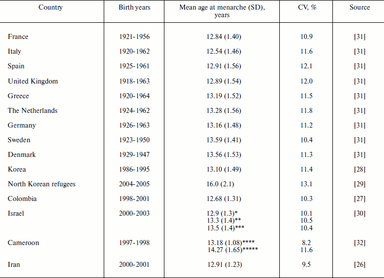
Age at menarche. Mean age at menarche in the studied human populations is in the range of 12-16 years (Table 1). Age at menarche demonstrates relatively low variability with standard deviations ranging from 1.1 to 2.1 years and coefficient of variation ranging from 8.2 to 13.1%. In a population with a history of poor nutrition (North Korean refugees), all measured characteristics – the mean age at menarche (16 years), its standard deviation (2.1 years), and coefficient of variation (13.1%) are particularly high compared to other populations [29]. It is likely that women in the prehistoric population had a higher variation of this ontogenesis characteristic than is observed now.
Table 1. Mean age at menarche and its
standard deviation (SD) and coefficient of variation (CV) in human
populations
*Obese women.
**Non-obese, non-lean women.
***Lean women.
****Urban areas.
*****Rural areas.
In addition to age at menarche, anthropologists have studied other characteristics of sexual maturity. For example, a study of sexual maturity among boys based on the NHANES III data demonstrated variability of age at complete maturity of genitalia, which was similar to variability of age at menarche for girls: range of 1.2-1.9 years for standard deviation [46].
Age at onset of menarche is an example of a characteristic determined by the ontogenesis program and is used as a marker of sexual maturity. Studies show that this developmental characteristic has a significant genetic component with heritability equal to about 0.49 [47, 48]. On the other hand, the age at menarche demonstrates environmental plasticity: in the last two centuries, age at menarche has decreased in several European populations [31]. Similar changes were observed in other countries [28, 49, 50], although recently further decline of the age at onset of menarche has stopped [51]. Age at menarche is negatively correlated with urbanization, socio-economic status, and body mass index [27, 30]. Earlier age of menarche is associated with higher total mortality as well as mortality from stroke and ischemic heart disease at adult ages [52].
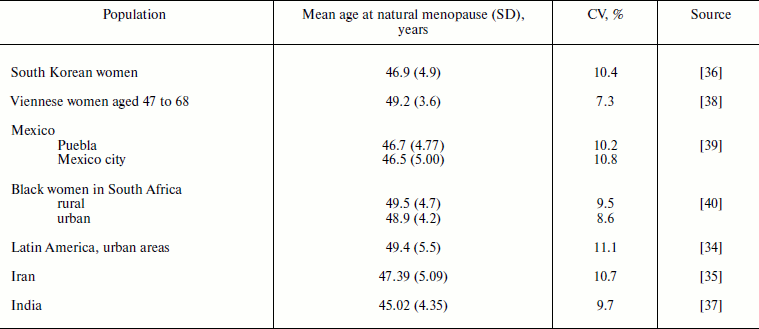
Age at natural menopause. Mean age at natural menopause in the studied human populations is in the range of 45-50 years (Table 2). Age at menopause has higher values of standard deviation compared to the age at menarche: 3.6-5.5 years. However, the relative measure of variability (coefficient of variation) is almost identical to the same measure for the age at menarche: 7.3-11.1%. Thus, both ages of starting reproduction and ages of cessation of reproduction in human populations show similar values of relative variability.
Table 2. Mean age at natural menopause, its
standard deviation (SD), and coefficient of variation (CV) in human
populations
Age at natural menopause is a hallmark of the end of reproduction related to the aging of the reproductive system [53]. Age at natural menopause shows slight increase over time. For example, in women in the United States the mean age at natural menopause increased by 17 months for those born between 1915 and 1939 (49.1 vs. 50.5 years; p = 0.001) [50]. Heritability of the age at menopause is similar to heritability of the age at menarche and is equal to 0.49 [54]. Lower age at menopause is associated with higher total mortality [55-57] and mortality from cardiovascular diseases, cancer, and external causes [36, 57].
Study of the representative sample of the United States population. Study of the MIDUS sample has an advantage of estimating both ages at menarche and menopause using the same group of women. The MIDUS sample consists of predominantly white women (over 85%). We used a subgroup of women aged 60 years and over, so that most of them were menopausal by the time of survey. Women reporting past hysterectomy were excluded from the analyses to avoid cases of surgical menopause.
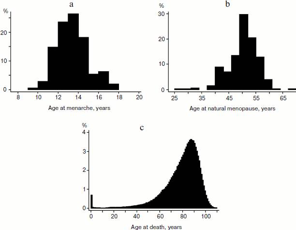
Figure 1a shows the distribution of women by reported age at menarche in the MIDUS sample. This distribution shows positive skewness equal to +0.56 with only a few cases having menarche below age 10 years. A positive skewness indicates that the tail on the right side of the distribution is longer than that on the left side, and the bulk of the values lie to the left of the mean value of 12.9 years. This may indicate that there are many environmental and genetic factors delaying sexual maturation, while it is far more difficult to accelerate it.
On the contrary, the distribution of age at natural menopause demonstrates negative skewness equal to –0.72 with few cases reporting menopause at ages over 60 years (Fig. 1b). A negative skewness indicates that the tail on the left side of the distribution is longer than that on the right side, and the bulk of the values (including the peak modal age) lie to the right of the mean of 49.7 years. This may indicate that there are many environmental and genetic factors accelerating reproductive aging, while it is far more difficult to delay it.Fig. 1. a) Distribution of age at menarche for women participating in the MIDUS study (United States). b) Distribution of age at natural menopause for women participating in the MIDUS study (United States). c) Distribution of age at death for women in the United States in 1995 (source: 1995 United States Life Table, Human Mortality Database).
Distribution of age at death (Fig. 1c) also demonstrates negative skewness similar to the distribution of the age at natural menopause. In this case, the skewness is equal to –1.81 (–1.26 for deaths at ages 10+ years).
Table 3 compares variability measures for distribution of age at menarche, age at menopause, and age at death for women in the United States. Note that coefficients of variation for ages at menarche and ages at menopause are quite similar. The coefficient of variation for age at death is two times higher than that for age at menarche (Table 3).
Table 3. Variation for characteristics of
human ontogenesis and aging (women in the United States)

Table 4 presents results of a comparative study of ages at menarche and death for women in Europe and the United States. Note that the standard deviations for ages at menarche are about 10 times lower than the standard deviations for ages at death. However, the coefficients of variation for ages at onset of menarche and ages at death for contemporary populations are of the same order of magnitude (Table 4).
Table 4. Variation of an ontogenesis
characteristic (age at menarche) and a characteristic related to aging
(age at death) for women in Europe and the United States
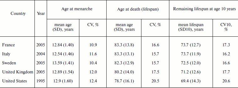
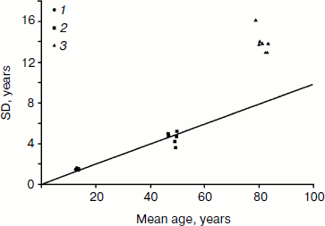
Figure 2 compares mean values (horizontal axis) and standard deviations (vertical axis) for all three studied characteristics: age at menarche, menopause, and death. This is a convenient way to visualize all the data on one graph and to infer relative variability (coefficient of variation) from the slope of the line connecting the plotted data with the origin point (the point at which the axes of a coordinate system intersect). Note that the relative variability of the measures characterizing both development and aging of the reproductive system is surprisingly the same (both sets of data are on the same line with zero intercept when extrapolated to zero mean value; the slope coefficient of this line is equal to the coefficient of variation). Relative variability of total lifespan (coefficient of variation) is about 1.5-2.0 times higher (this set of data is far above the line). However, we need to remember that distribution of total deaths includes so-called non-natural deaths from external causes (accidents, suicides, etc.). Variability is also increased when deaths of infants and children are taken into account. Demographers now use standard deviation at age 10 years to evaluate the distribution of lifespan at older ages. The age of 10 years represents the age when mortality starts to increase, and hence this age indicates the beginning of manifestation of the aging process. If we use estimates of standard deviation at age 10 (SD10), then we get lower values for standard deviation, but not for coefficient of variation (Table 4).
Thus, coefficients of variation (measures of relative dispersion) for an ontogenesis characteristic (menarche) and aging characteristics (menopause and death) are rather close to each other. This is particularly true for characteristics related to sexual maturation and reproductive aging: ages at menarche and ages at menopause have surprisingly similar relative variability. Some gerontologists believe that a programmed process should include stereotypical steps [1]. Interestingly, both ontogenesis and aging of the female reproductive system in humans can be considered as examples of rather stereotypical behavior.Fig. 2. Comparison of mean ages at menarche (1), menopause (2), and death (3) as well as their standard deviations for studied human populations. Mean values are presented on the horizontal axis and standard deviations on the vertical axis. Data are taken from Tables 1-4.
To summarize, this study has found a surprising precision of a “non-existent” aging program [7, 25]: relative variability for reproductive aging (menopause) is the same as for “programmed” sexual maturation (menarche).
We would like to thank participants of the international scientific workshop “From Homo sapiens to Homo sapiens liberatus” (May, 2010, Moscow State University, Russia) for their useful comments and suggestions made in response to our related presentation there.
The authors are grateful to the Rostok Group (Mr. A. V. Chikunov, Founder and President) and the Institute of Mitoengineering of Moscow State University for financial support. Also, this study was supported in part by the National Institute on Aging (R01 AG028620 grant for L.G.).
REFERENCES
1.Austad, S. N. (2004) Aging Cell, 3,
249-251.
2.Bredesen, D. E. (2004) Aging Cell, 3,
261-262.
3.Gavrilov, L. A., and Gavrilova, N. S. (1991) The
Biology of Life Span: A Quantitative Approach, Harwood Academic
Publisher, New York.
4.Gavrilov, L. A., and Gavrilova, N. S. (2006) in
Handbook of the Biology of Aging (Masoro, E. J., and Austad, S.
N., eds.) Academic Press, San Diego, pp. 1-40.
5.Kirkwood, T. B. L., Feder, M., Finch, C. E.,
Franceschi, C., Globerson, A., Klingenberg, C. P., LaMarco, K., Omholt,
S., and Westendorp, R. G. J. (2005) Mechanisms Ageing Devel.,
126, 439-443.
6.Gavrilov, L. A., and Gavrilova, N. S. (2002)
Thescientificworldjournal, 2, 339-356.
7.Bredesen, D. E. (2004) Aging Cell, 3,
255-259.
8.Mitteldorf, J. (2010) Rejuvenation Res.,
13, 322-326.
9.Blagosklonny, M. V. (2007) J. Cell.
Biochem., 102, 1389-1399.
10.Bowles, J. (2000) Med. Hypotheses,
54, 326-339.
11.Bowles, J. T. (1998) Med. Hypotheses,
51, 179-221.
12.De Magalhaes, J. P., and Church, G. M. (2005)
Physiology, 20, 252-259.
13.Goldsmith, T. C. (2003) Aging as an Evolved
Characteristic - Weismann’s Theory Reconsidered. The
Evolution of Aging, Universe Publishers, New York.
14.Goldsmith, T. C. (2008) J. Theor. Biol.,
252, 764-768.
15.Libertini, G. (2008)
Thescientificworldjournal, 8, 182-193.
16.Longo, V. D., Mitteldorf, J., and Skulachev, V.
P. (2005) Nature Rev. Genet., 6, 866-872.
17.Pierpaoli, W., and Bulian, D. (2001) J.
Anti-Aging Med., 4, 31-37.
18.Skulachev, V. P. (1997) Biochemistry
(Moscow), 62, 1191-1195.
19.Skulachev, V. P. (1999) Biochemistry
(Moscow), 64, 1418-1426.
20.Skulachev, V. P. (1999) Mol. Asp. Med.,
20, 139-184.
21.Skulachev, V. P. (2001) Exp. Gerontol.,
36, 995-1024.
22.Skulachev, V. P. (2003) in Topics in Current
Genetics Model Systems in Ageing (Nystrom, T., and Osiewacz, H. D.,
eds.) Springer-Verlag, Berlin-Heidelberg, pp. 191-238.
23.Skulachev, V. P. (2009) Biochim. Biophys.
Acta-Bioenergetics, 1777, S6-S6.
24.Skulachev, V. P., and Longo, V. D. (2005)
Reversal of Aging: Resetting the Pineal Clock, 1057,
145-164.
25.Austad, S. N. (2004) Aging Cell, 3,
253-254.
26.Ayatollahi, S. M. T., Dowlatabadi, E., and
Ayatollahi, S. A. R. (2002) Ann. Hum. Biol., 29,
355-362.
27.Chavarro, J., Villamor, E., Narvaez, J., and
Hoyos, A. (2004) Ann. Hum. Biol., 31, 245-257.
28.Cho, G. J., Park, H. T., Shin, J. H., Hur, J. Y.,
Kim, Y. T., Kim, S. H., Lee, K. W., and Kim, T. (2010) Eur. J.
Pediatrics, 169, 89-94.
29.Ku, S. Y., Kang, J. W., Kim, H., Kim, Y. D., Jee,
B. C., Suh, C. S., Choi, Y. M., Kim, J. G., Moon, S. Y., and Kim, S. H.
(2006) Hum. Reprod., 21, 833-836.
30.Mandel, D., Zimlichman, E., Mimouni, F. B.,
Grotto, I., and Kreiss, Y. (2004) J. Pediatr. Endocrinol.
Metab., 17, 1507-1510.
31.Onland-Moret, N. C., Peeters, P. H. M., van Gils,
C. H., Clavel-Chapelon, F., Key, T., Tjonneland, A., Trichopoulou, A.,
Kaaks, R., Manjer, J., Panico, S., et al. (2005) Am. J.
Epidemiol., 162, 623-632.
32.Pasquet, P., Biyong, A. M. D., Rikong-Adie, H.,
Befidi-Mengue, R., Garba, M. T., and Froment, A. (1999) Ann. Hum.
Biol., 26, 89-97.
33.Brim, O. G., Ryff, C. D., and Kessler, R. C.
(2004) in How Healthy Are We?: A National Study of Well-Being at
Midlife, University of Chicago Press, Chicago, pp. 1-34.
34.Blumel, J. E., Chedraui, P., Calle, A., Bocanera,
R., Depiano, E., Figueroa-Casas, P., Gonzalez, C., Martino, M., Royer,
M., Zuniga, C., et al. (2006) Menopause – J. North Amer.
Menopause Soc., 13, 706-712.
35.Fallahzadeh, H. (2007) Menopause – J.
North Amer. Menopause Soc., 14, 900-904.
36.Hong, J. S., Yi, S. W., Kang, H. C., Jee, S. H.,
Kang, H. G., Bayasgalan, G., and Ohrr, H. (2007) Maturitas,
56, 411-419.
37.Kapur, P., Sinha, B., and Pereira, B. M. J.
(2009) Menopause – J. North Amer. Menopause Soc.,
16, 378-384.
38.Kirchengast, S. (1994) Homo, 44,
263-277.
39.Sievert, L. L., and Hautaniemi, S. I. (2003)
Hum. Biol., 75, 205-226.
40.Walker, A. R. P., Walker, B. F., Ncongwane, J.,
and Tshabalala, E. N. (1984) Br. J. Obstetrics Gynecol.,
91, 797-801.
41.Human Mortality Database (2010) http://www.mortality.org, Accessed 02/14/10,
University of California, Berkeley, Max Planck Institute for
Demographic Research.
42.Kessler, R. C., DuPont, R. L., Berglund, P., and
Wittchen, H. U. (1999) Am. J. Psychiatry, 156,
1915-1923.
43.Kessler, R. C., Mickelson, K., and Zahao, S.
(1997) Social Policy, 27, 27-46.
44.Edwards, R. D., and Tuljapurkar, S. (2005)
Population Devel. Rev., 31, 645-674.
45.Simpson, G. G., Roe, A., and Lewontin, R. G.
(2003) Quantitative Zoology: Revised Edition, Dover
Publications, Inc., New York.
46.Sun, S. M. S., Schubert, C. M., Chumlea, W. C.,
Roche, A. F., Kulin, H. E., Lee, P. A., Himes, J. H., and Ryan, A. S.
(2002) Pediatrics, 110, 911-919.
47.Towne, B., Czerwinski, S. A., Dernerath, E. W.,
Blangero, J., Roche, A. F., and Siervogel, R. M. (2005) Am. J. Phys.
Anthropol., 128, 210-219.
48.Salces, I., Rebato, E. M., Susanne, C., San
Martin, L., and Rosique, J. (2001) Ann. Hum. Biol., 28,
143-156.
49.Hwang, J. Y., Shin, C., Frongillo, E. A., Shin,
K. R., and Jo, I. (2003) Ann. Hum. Biol., 30,
434-442.
50.Nichols, H. B., Trentham-Dietz, A., Hampton, J.
M., Titus-Ernstoff, L., Egan, K. M., Willett, W. C., and Newcomb, P. A.
(2006) Am. J. Epidemiol., 164, 1003-1011.
51.Helm, P., and Gronlund, L. (1998) Acta
Obstetr. Gynecol. Scand., 77, 198-200.
52.Jacobsen, B. K., Oda, K., Knutsen, S. F., and
Fraser, G. E. (2009) Int. J. Epidemiol., 38, 245-252.
53.Velde, E. R. T., Dorland, M., and Broekmans, F.
J. (1998) Maturitas, 30, 119-125.
54.Murabito, J. M., Yang, Q., Fox, C., Wilson, P. W.
F., and Cupples, L. A. (2005) J. Clin. Endocrinol. Metab.,
90, 3427-3430.
55.Amagai, Y., Ishikawa, S., Gotoh, T., Kayaba, K.,
Nakamura, Y., and Kajii, E. (2006) J. Epidemiol., 16,
161-166.
56.Jacobsen, B. K., Heuch, I., and Kvale, G. (2003)
Am. J. Epidemiol., 157, 923-929.
57.Mondul, A. M., Rodriguez, C., Jacobs, E. J., and
Calle, E. E. (2005) Am. J. Epidemiol., 162,
1089-1097.
