REVIEW: Sex and Aging: A Comparison between Two Phenoptotic Phenomena
Giacinto Libertini
Independent researcher, member of the Italian Society for Evolutionary Biology, Italy; E-mail: giacinto.libertini@tin.it
Received June 2, 2017
Phenoptosis is a phenomenon that is genetically programmed and favored by natural selection, and that determines death or increased risk of death (fitness reduction) for the individual that manifests it. Aging, here defined as age-related progressive mortality increase in the wild, if programmed and favored by natural selection, falls within the definition of phenoptosis. Sexual reproduction (sex), as for the involved individuals determines fitness reduction and, in some species, even certain death, also falls within the definition of phenoptosis. In this review, sex and aging are analyzed as phenoptotic phenomena, and the similarities between them are investigated. In particular, from a theoretical standpoint, the genes that cause and regulate these phenomena: (i) require analyses that consider both individual and supra-individual selection because they are harmful in terms of individual selection, but advantageous (that is, favored by natural selection) in particular conditions of supra-individual selection; (ii) determine a higher velocity of and greater opportunities for evolution and, therefore, greater evolutionary potential (evolvability); (iii) are advantageous under ecological conditions of K-selection and with finite populations; (iv) are disadvantageous (that is, not favored by natural selection) under ecological conditions of r-selection and with unlimited populations; (v) are not advantageous in all ecological conditions and, so, species that reproduce asexually or species that do not age are predicted and exist.
KEY WORDS: aging, sex, phenoptosis, supra-individual selection, K-selection, r-selectionDOI: 10.1134/S0006297917120045
For many years, the justifications in evolutionary terms of sex and aging (that is, of the genes that cause and regulate these phenomena) have been subjects of much debate. A complete analysis and discussion of the theories about the evolutionary causes of each of the two phenomena is beyond the scope of this review.
Instead:
– regarding sex, the attention is focused mainly on a model based on the old hypothesis that its evolutionary advantage derives from the recombination of the parents’ genes in their offspring. However, sex cannot be advantageous (that is, favored by natural selection) in condition of r-selection [1] and in numerically unlimited populations;
– regarding aging, the analysis is focused on the hypothesis that aging is advantageous because it brings about a quicker generational turnover, which leads to a greater speed of evolution. However, aging may only be favored, by supra-individual selection, under ecological conditions of K-selection [1] and in species that are divided into small demes.
Then, for both phenomena, the predictions of the aforesaid hypotheses about their existence among the various species, depending on ecological conditions, will be expounded and briefly compared with the predictions of other hypotheses.
Finally, the nature of sex and aging as phenoptotic phenomena and a general comparison between the two phenomena will be outlined.
SEX
The advantage of sex. The evolutionary justification of gene recombination between two individuals (defined as “mixis” or “amphimixis”, or commonly as “sex”), is a much-debated topic [2-16].
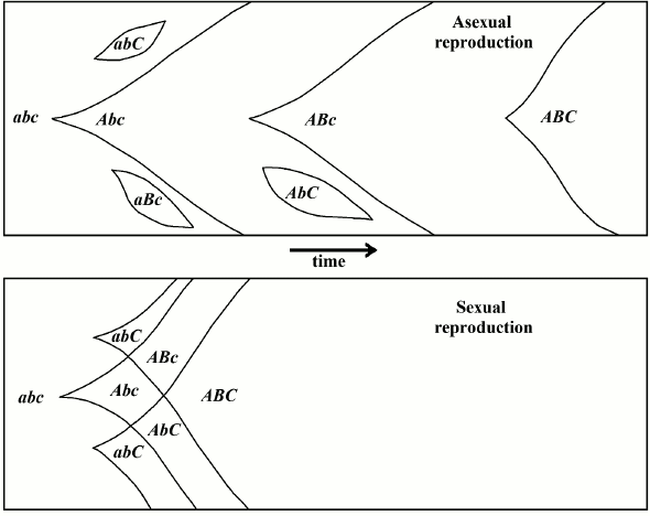
The “classic” hypothesis, also known as the Fisher–Muller hypothesis or, by using Bell’s old eponym, “The Vicar of Bray” [5], maintains that sex is evolutionarily advantageous because it allows for a continuous rearrangement of genes in any offspring (Fig. 1). This thesis was first expressed by Weismann [17] and by Guenther [18]. It was later described from a population genetics perspective by Fisher [19] and Muller [20], and afterwards, with greater mathematical detail, by Muller [21, 22] and Crow and Kimura [23].
Fig. 1. In the “classic” hypothesis, sex would be advantageous from an evolutionary perspective because it allows for the continuous rearrangement of genes and, therefore, the attainment of the best combinations in a shorter period of time earlier compared to asexual reproduction (redrawn from [23]).
Maynard Smith [4, 24] criticized the “classic” hypothesis with the following simple but effective argument.
If, in an infinite population of a haploid species, there are two genes (a, b), with alleles (A, B) that have an advantage (sA, sB) over a and b, respectively, the combination frequencies in the next generation will be:
Pn+1,ab = Pn,ab/T
Pn+1,Ab = Pn,Ab (1 + sA)/T
Pn+1,aB = Pn,aB (1 + sB)/T
Pn+1,AB = Pn,AB (1 + sAB)/T, (1)
where
sAB (advantage of AB over ab) = [(1 + sA)(1 + sB) – 1] k, (2)
k = interaction between the fitnesses (epistasis); Pn,xy = frequency of xy combination at generation n; and T = the sum of the numerators.
If there is no linkage disequilibrium (D) at generation n, that is, if:
D = Pn,ab Pn,AB – Pn,Ab Pn,aB = 0 (3)
with no epistasis (k = 1), then the group of formulas above (1) determines that in the next generation it will always be:
D = Pn+1,ab Pn+1,AB – Pn+1,Ab Pn+1,aB = 0 (4)
with or without recombination, which can only halve linkage disequilibrium at each generation [4]. Therefore, with these conditions, sex cannot be advantageous.
With negative linkage disequilibrium (D < 0) sex would be advantageous, with positive linkage disequilibrium sex would be disadvantageous [4].
If there is positive epistasis (k > 1), sex is disadvantageous because it breaks the more advantageous combination (AB); the contrary happens if there is negative epistasis (k < 1). However, there is no justification to assume that, in the real world, epistasis should be in general positive and, therefore, sex advantageous [4].
Maynard Smith tried to overcome his argument by observing that it was valid for infinite populations, but that linkage disequilibria should arise by chance in finite populations [4], and so, in conditions of negative linkage disequilibrium, sex would be advantageous, as previously observed by Felsenstein [25].
Many scholars did not accept the counterarguments of Maynard Smith [3, 26] and the doubts about the validity of the “classic” explanation of sex, defined here as the “S1” hypothesis, caused alternative hypotheses to flourish. For example, to use the eponyms of Bell [5]:
S2) Muller’s ratchet hypothesis [12, 22, 25, 27-31]. For this theory, sex facilitates the elimination of unfavorable mutations. Without mixis, damaging mutations would continually accumulate in a population, causing a decline of its mean fitness [28];
S3) Best-Man hypothesis [32-35]. Recombination may produce individuals with extraordinarily high fitness. If these individuals have an appreciable chance of surviving in conditions where all the others die, then they will have a greater proportion of progeny in the next generation;
S4) Hitch-hiker hypothesis [25, 36]. Stochastically generated linkage disequilibria increase the variance of fitness for any single-locus genotype and, therefore, slow the fixation of a favorable allele. An allele that increases the rate of recombination reduces the linkage disequilibria and accelerates the fixation of favorable alleles. Thus, for the effects of selection, it is hitch-hiked by these favorable alleles;
S5) Tangled-Bank hypothesis [2, 6, 37-40]. Sex diversifies progeny, and its advantage is greater in conditions of environmental spatial heterogeneity, that is, if there are various “ecological niches in the same small geographical area – in an environment which does not change in time” [5];
S6) Red Queen hypothesis [5, 6, 41-55]. This popular theory maintains that sex has evolved “in response to the shifting adaptive landscape generated by the evolution of interacting species” [50]; “The Red Queen Hypothesis … suggests that the coevolutionary dynamics of host-parasite systems can generate selection for increased host recombination… A prerequisite for this mechanism is that host-parasite interactions generate persistent oscillations of linkage disequilibria…” [51];
S7) Historical hypothesis [3]. There is no evolutionary cause for sex. Sexual or asexual condition of a species is mainly determined by the sexuality or asexuality of the ancestor species;
and, moreover, the hypotheses that:
S8) Sex is advantageous because it slows evolution and excessive specialization [3, 56];
S9) Recombination eliminates the negative linkage disequilibria generated by synergistic epistasis [57-60];
S10) More than one theory is necessary to explain the existence of sex [61];
and other theories, which have been classified by Kondrashov [62].
There are many well-known criticisms of these hypotheses [5]. Moreover, some attempts to explain the advantage of sex in finite populations appear too complex [63-69], and the evolutionary advantage of sex should be investigated without hypothesizing artful mechanisms.
However, it is possible to define a model that shows sex – in terms of individual selection, as considered necessary by Felsenstein [25] – as both advantageous in finite populations and not advantageous in infinite populations. Such a model takes into account: (i) the important observation expressed by Felsenstein: “… those authors who have allowed finite-population effects into their models have been the ones who found an advantage to having recombination, while those whose models were completely deterministic found no consistent advantage…” [25]; and (ii) the suggestion that real populations are subject to genetic drift and are spatially structured [70].
The simulation model for infinite populations. Let us consider a species that is: a) haploid; b) with an infinite population; c) with half of the individuals at generation zero having – in a specific locus – a gene R+ allowing conjugation and free recombination with all other individuals having R+, while the others have an allele R– allowing conjugation and recombination only in a fraction (z) of individuals. If z > 0, the pool of recombinant individuals is constituted of all R+ individuals plus a fraction z of R– individuals. However, if z = 0, as in most of the following simulations, there is “no sharp distinction between individual selection and group selection”, as highlighted by Felsenstein and Yokoyama [71]. In any case, the selection will be considered only in strict terms of individual selection;
d) with R+ and R– individuals having the same ecological niche and being by no means distinguishable except for the condition expressed above in (c);
e) with zero frequency of mutation rates for turning R+ into R–, namely turning a sexual individual into an asexual individual, or vice versa;
f) with the disadvantage for sexual individuals of finding a mate and of coupling and with any other possible disadvantage of sex, the so-called “cost of sex” included, here not considered;
g) with new alleles (A, B, C, …) more advantageous than those alleles that prevail in the species (a, b, c, …) and, in the simulations, are supposed at generation zero to have a frequency equal to 1;
h) with independent gene transmission of any allele, that is, the recombination fraction is assumed to be equal to 0.5;
i) with the mutation rate, at each generation, of an allele x into X equal to ux and the back-mutation rate of X into x equal to wx.
The question is whether sexual individuals have an advantage over asexual individuals, or vice versa, that is, whether there is a spreading or a decay of R+.
The model is restricted to the cases of:
(1) two genes (a, b) and their respective new alleles (A, B) (“2G case”), with four possible combinations (ab, Ab, aB, AB); and,
(2) three genes (a, b, c) and their respective new alleles (A, B, C) (“3G case”), with eight possible combinations (abc, Abc, aBc, abC, ABc, aBC, AbC, ABC).
These restrictions are not a limitation because, if sex proves to be advantageous with only two or three genes, the greater fitness will be self-evident with more genes.
For the sake of simplicity, it is hypothesized that:
u = ua = ub = uc, (5)
w = wa = wb = wc, (6)
s = sA = sB = sC. (7)
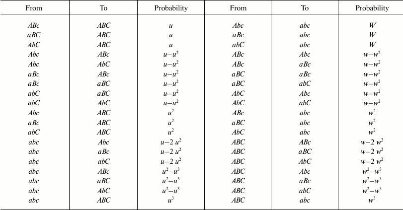
With two and three genes, the possible cases of transformation by mutations from one combination into another and the probability of each transformation are indicated in Fig. 2 and Tables 1 and 2.
Fig. 2. Possible transformations of one combination into another in the 2G case (A) and in the 3G case (B).
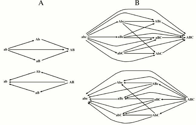
Table 1. Possible transformations of
one combination into another and their probabilities in the 2G case
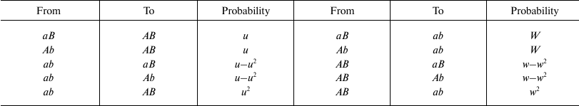
Table 2. Possible transformations of
one combination into another and their probabilities in the 3G case
The fitness for individuals with two advantageous alleles (FXY; XY means AB, for the 2G case; AB or BC or AC, for the 3G case) is:
FXY = 1 + k [(1 + s)2 – 1], (8)
where k = 1, when there is no interaction, or epistasis, between the genes.
In the case of three advantageous alleles:
FABC = 1 + k2 [(1 + s)3 – 1]. (9)
If we indicate the frequency of the combination xy in R+ individuals at the n-th generation with Pxy,n and in R– individuals with Pxy’,n, the recombination for R+ individuals is simulated, in the 2G case, by calculating the frequencies of a, A, b, and B, over the total number of individuals with R+ (PR+):
Pa,n = Pab,n + PaB,n, (10)
and then by using the equations:
Pab,n+1 = ½ Pab,n + ½ Pa,n Pb,n PR+,n. (11)
PR+,n PR+,n
The first part of each Eq. (11) means that, when recombination occurs between individual I and another individual, in half of the cases, the allele present in I does not change (see condition “h” above). The second part means that, in the remaining half of the cases, the allele present in I is substituted by another allele from the other individual. The frequencies of the substituting alleles are given by the multiplication of the relative frequencies of each allele (Px,n/PR+,n), with the result multiplied for the frequency of R+ (PR+,n).
On the contrary, for R– individuals and when z = 0 (see condition “c” above), there is no calculation:
Pab’,n+1 = Pab’,n. (12)
For the 3G case, recombination for R+ individuals is simulated by calculating the frequencies of a, A, b, B, c, and C over the total number of individuals with R+:
Pa,n = Pabc,n + PaBc,n + PabC,n + PaBC,n; (13)
and then by using the equations:
Pabc,n+1 = ½ Pabc,n + ½ Pa,n Pb,n Pc,n PR+,n; (14)
PR+,n PR+,n PR+,n
while for R– individuals:
Pabc’,n+1 = Pabc’,n. (15)
The simulation model for finite populations. All of the equations above are correct in the abstract case of an infinite population, but real-life populations are made up of N individuals, with N being a finite integer number, and are subject to random fluctuations for N and for each gene combination present therein.
At each generation, an allele, x, may be transformed into another allele, X, with a probability equal to the frequency of mutation ux. Therefore, depending on the value of ux, the frequencies of x and X at generation n (Px,n and PX,n) are expected to pass to the frequencies Px,n+1 and PX,n+1 in the next generation with a difference of Δx = –ux Px,n and of ΔX = +ux PX,n, respectively.
More generally, because of mutations, advantages, recombination, genetic drift, and other causes, the frequency of a combination xy is expected to pass from Pxy,n to Pxy,n+1 in the next generation with a difference Δxy in absolute value between Pxy,n to Pxy,n+1.
For real populations, Δxy values, multiplied by N, must always be integer numbers.
In the simulation model, each of these integer numbers is obtained using the “rbinom” function of the package R of The R Foundation for Statistical Computing© (http://www.r-project.org/), which generates random deviate integers.
The function is used in the program to simulate the variations in the frequencies due to: mutations (for example, a → A); back-mutations (for example, A → a); advantages; recombination; genetic drift; the diffusion of combinations among demes, when the population is not composed of a single deme (d = 1), but of several demes (d > 1), each composed of N individuals and with a mean interdemic diffusion of genes at each generation equal to f.
At each generation, the function is used several times (up to 13,000 times in 3G case and 100 demes).
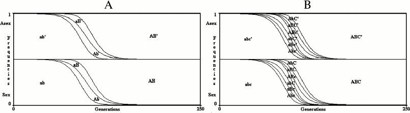
Results for an infinite population. With no epistasis (k = 1) and no linkage disequilibrium (D = 0), sex is neutral with any value of u, w or s (Fig. 3).
In Fig. 3, the value of R+ after 250 generations (PR+,250) is 0.499997620408316 for the 2G case and 0.499998194700698 for the 3G case. The slight differences between these values and 0.5 (the frequency of R+ at generation 0) are due to the little positive linkage disequilibria caused by mutations. The frequencies of both R+ and R– at generation 0 (PR+,0; PR–,0) are 0.5 to give to sex and asexual individuals the same starting conditions. With any other value as well (for example, PR+,0 = 0.6; PR–,0 = 1 – PR+,0 = 0.4), the model shows that in infinite populations there is no significant variation from the initial frequencies of R+ and R–, as predicted by Maynard Smith [4]. The simulations, in all the figures, have been extended up to 250 generations, which is sufficient to stabilize the frequencies of combinations and R+ values.
Fig. 3. The model shows no advantage for sex in infinite populations in 2G case (A) and 3G case (B). The results of the model are greatly altered by any possible modification of the formulas shown in Table 1 or Table 2, which always causes a strong prevalence of one of the two conditions.
With any time-dependent variation of the value of s, sex is neutral (Fig. 4), that is, any oscillating value of s that is due to changing interactions between species cannot justify sex. This result must be stressed and deepened. The Red Queen hypothesis rightly underlines the likely concept that biotic factors are quantitatively more important selective forces compared to physical factors. The Red Queen hypothesis is deduced from this concept (here defined the “Red Queen concept”), which is probably true considering the numberless interactions between different species (for example, predator–prey, herbivore–grass, parasite–host, host–commensal species, cooperative species, and competitors for the same resources) and because in many cases these interactions cause oscillating values for the selective pressures [5, 50, 51].
Fig. 4. In the simulations of a 2G case (A) and a 3G case (B), s value oscillates from –0.1 to +0.1 every 150 generations. The model shows no advantage for sex in infinite populations if there are oscillating values of s.
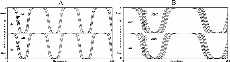
In contrast to the results for infinite populations, the results for finite populations (described in the next section) show that sex is advantageous. However, this is in relation to how finite and discrete a real population is, not because of the biotic or physical character of selective pressures or of the condition of oscillating values of any advantage (s > 0) or disadvantage (s < 0). This should not be interpreted as a negation or diminution of the “Red Queen concept” but as a theoretical strong argument against the Red Queen hypothesis.
If k > 1 (positive epistasis), sex is disadvantageous; if k < 1 (negative epistasis), sex is advantageous. If D > 0 (positive linkage disequilibrium), sex is disadvantageous; if D < 0 (negative linkage disequilibrium), sex is advantageous (see Supplement A to this paper on the site of the journal (http://protein.bio.msu.ru/biokhimiya) and Springer site (Link.springer.com)). However, in an unlimited population, a justification for sex based on prevailing conditions of negative epistasis or of negative linkage disequilibrium is unlikely.
In an infinite population, the results of the simulation model confirm the considerations obtained through analytical arguments by various authors [24, 72-74].
Results for a finite population. Examples of single simulations are illustrated in Fig. 5. When N (the number of individuals) is small, the simultaneous appearance of two advantageous mutations is rare and sex cannot be favored. The prevalence of R+ or R– is determined only by genetic drift (that is, by chance).
Fig. 5. 2G case, single simulations in finite populations. A) log10N = 2; B) log10N = 5; C) log10N = 6; D) log10N = 9. In the case (A), only genetic drift determines the fluctuation of R+ and R– values. In the cases (B), (C), and (D), the prevalence of R+ or R– is determined by the random antecedence of mutation onset in R+ or R–.
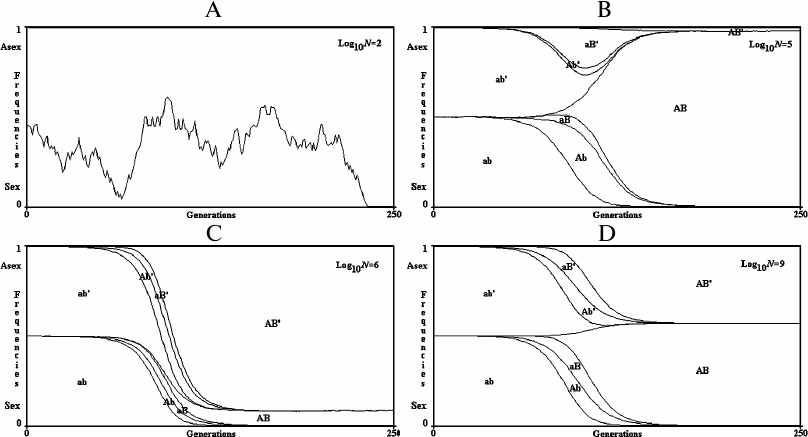
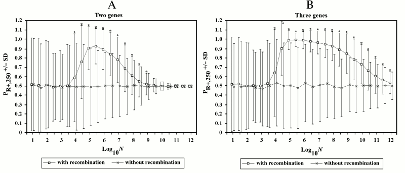
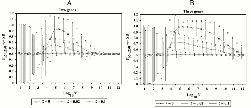
Figure 6 illustrates a series of simulations (1000 for each point) with log10N varying from 1 to 12 and increments of its value equal to 0.5. The mean (indicated by a square) and standard deviation (SD) are reported for each point and compared with another series of simulations (indicated by the symbol x) in which R+ individuals are not allowed to recombine. Each point is marked by an asterisk if the results are significantly different (t-test for two unpaired groups of data [75], p < 0.001).
In the 2G case, starting from values of log10N around 4, sex results to be generally favored, though often sex loses. With values of log10N greater than 5.5, the advantage (difference between PR+,250 and 0.5) becomes progressively smaller.
In the 3G case, the decline of sex advantage starts from greater values of log10N and is much slower.
Fig. 6. The effects of recombination in finite populations in 2G case (A) and 3G case (B). In this and subsequent figures, if not otherwise specified, the following conditions hold: u = w = 0.00001; s = 0.1; k = 1; and D = 0. The mean and standard deviation (SD) are reported for each point. For the series of simulations with recombination, an asterisk indicates a significant difference (p < 0.001) for each point compared to the corresponding point of simulations without recombination. In this and in subsequent figures, to avoid the superimposition of SD bars, the symbols of the first and of the second series have been shifted slightly to the left and to the right, respectively. Also, the results are always those obtained during the first runs of the simulations. (Repetitions of the simulation for each series gave results that were equivalent to those of the first runs. However, these results have not replaced those of the first runs.)
In Fig. 7, the series of simulations presented in Fig. 6 are compared with two other series of simulations in which recombination is allowed for a fraction (z) of R– individuals (see Supplement B to this paper on the site of the journal (http://protein.bio.msu.ru/biokhimiya) and Springer site (Link.springer.com) for the modifications of Eqs. (10)-(15) that are necessary when z > 0). Even when the values of z are small, the advantage of R+ over R– individuals fades.
Fig. 7. Effects of the variations of z in 2G case (A) and 3G case (B). The two series with z = 0 are the same as in Fig. 6 with recombination. When z = 0.02, the advantage for R+ individuals is greatly reduced, and when z = 0.1, there is no advantage. In this and in the subsequent figures, an asterisk or a cross indicate a significant difference (p < 0.001 and p < 0.01, respectively) for each point compared to the corresponding point of simulations without recombination in Fig. 6, A and B.
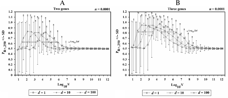
In Fig. 8, the population (now defined as metapopulation) is divided into d demes, each composed of N individuals, with an interdemic interchange of individuals (f) equal to 0.1 per generation. The results show that, in terms of the advantage of sex, a metapopulation is equivalent to a single population of d·N individuals.
Fig. 8. Effects of the variations of d in 2G case (A) and 3G case (B). When there is an increase of d, there is a shift to the left in both sides of the curve. The shift is proportional to log10Δd.
Disadvantage of sex. Sexual individuals suffer from the disadvantages deriving from the search of a mate and related to the coupling. “Amphimicts [that is, individuals of sexual species] have one… handicap: they must be able to find a mate, and this may be an expensive, risky and time-consuming process” ([5], p. 357). Courtship and copulation take time and involve risks for life, which may be considered a form of optional phenoptosis [76].
In some species, death during or after mating is obligatory.
For example, sexual cannibalism “occurs in various arthropod taxa” [77], in particular among insects, arachnids and amphipods [78]. The males of Araneus, Argiope, and Crytophria (species of arachnids) are killed by the female during mating [79], and there are also cases of sexual cannibalism in copepods and gastropods [80]. The phenomenon, which is a clear form of obligatory phenoptosis [76] associated to mating, is considered adaptive [77], because “Sexual cannibalism had direct and positive effects on female fitness, as sexually cannibalistic females exhibited increased fecundity irrespective of their size, condition, and foraging rate. Male consumption was almost complete and represented a relevant food intake to females. We interpret sexual cannibalism as a strategic foraging decision…” [81].
In this work, these handicaps will be defined on the whole as “disadvantage of sex” (DS). The existence of the DS allows the definition of sex as a form of phenoptosis, which is obligatory in some cases and optional in most other cases, according to the definition of phenoptosis proposed elsewhere [76].
It is important to consider the DS because it hinders the spread of sex: clearly, if the DS is greater than the advantage of sex, mixis cannot be favored by natural selection.
The DS will be greater in severely disturbed habitats and in conditions of r-selection. As a matter of fact, in severely disturbed habitats the search for a mate is too expensive and risky. Likewise, in conditions of r-selection and in phases of exponential growth of population the crucial factor is the swiftness of reproduction, and sex, a “time consuming process” [5], is highly disadvantageous.
Given these considerations, Gerritson’s opinion that DS is greater under conditions of low population density [82] and, so “reproduction following long-distance dispersal should be parthenogenetic” ([5], p. 357), perhaps cannot be shared, because there is no severely disturbed habitat. On the contrary, as a matter of fact “parthenogenetic insects… very often live in small patches of high local population density” ([5], p. 357), which is a condition of r-selection.
A comparison between the empirical data and the predictions of various hypotheses that attempt to explain the evolutionary causes of sex is presented and discussed in the next section. Before this comparison, it is worth mentioning a popular topic that is a source of misunderstandings and incorrect conclusions.
The fact that “a copy of a given gene is certain to be present in any asexual egg, but has only a 50% chance of occurring in any given sexual ovum” [5], has been described as “cost of sex” [83], or “cost of meiosis” [3] or “twofold selective advantage” of parthenogenesis [4]. This creates doubts about the possibility that the advantage of sex could overcome this enormous cost (50% at each generation) to justify the existence of sex in evolutionary terms [84].
However, along these lines, for a man who produces millions of spermatozoa every day and is only successful in having with his partner a child with half of his genes every few years, and similarly for the many species of animals and plants that spread many eggs, spermatozoa, and seeds while only few are fertilized, or fertilize, we should speak of a “billion-fold selective cost of sex”. This type of reasoning would make unlikely to find for sex an evolutionary advantage of the same weight that could justify its existence.
More accurately, the reasoning should compare the quantity of resources invested with the number of successful offspring obtained.
It is easy to show that in the particular and very simple case of isogamous species (that is, species with gametes of equal size), the “cost of sex” does not exist.
Indeed, in the case of an isogamous species, if m is the optimal size of a zygote, the production of a single asexual zygote of m size has a cost proportional to m. This cost is equal to the cost of two sexual gametes of size m/2 such that, when coupled with two other gametes of the same size, the optimal size m for two zygotes is obtained. In both cases, a gene has the same probability of being present in a zygote (1 in the first case; 0.5 × 2 = 1 in the second case).
This is true if the relationship between zygote size and viability is linear. In fact, if we symbolize survival with s, the relationship between zygote size and its viability can be expressed as m = AsB, where A and B are constants. In the model proposed by some authors [85-87], for isogamous species, when B = 1 (linear relationship between zygote size and viability), the overall cost of sex is zero; when B < 1, the cost of sex is > 0, and when B > 1, the cost of sex is < 0 [5]. This means that for isogamous species, only in particular conditions (B < 1), there is a cost of sex; in other conditions (B ≥ 1), the cost of sex is an advantage or is non-existent.
Therefore, in general, for isogamous species the cost of sex is non-existent, although in some particular cases (when B ≠ 1), an advantage or a disadvantage could exist.
However, for most species there are many differences between female and male individuals, and between their roles and their investment of resources in sexual reproduction, which must be considered as extreme forms of anisogamy. If, in the evolution from isogamy to any form of anisogamy, there are certainly advantages and disadvantages caused by anisogamy, they are related to anisogamy and not to sex in and of itself. For example, the phenomenon of “males with the exaggerated sexually selected characters [that] are more attractive to females” [88] has been subject of much debate [88-90], but this “handicap” [88] is clearly related to sexual differentiation and not to sex in and of itself.
In any case, the critical factor is not simply the number of DNA copies invested by each parent, but the ratio between the amount of resources invested by the two parents and the number of successful offspring.
A comparative and experimental critique of the theories (empirical evidence for the predictions of various theories). As a theory is sound or unsound according to whether its predictions are confirmed or disproved by empirical data, it is necessary to verify whether predictions of the “classic” hypothesis and of other hypotheses about the evolutionary advantage of sexual reproduction are confirmed or disproved by data from natural observation.
In Table 3, the predictions of the “classic” hypothesis and those of three other hypotheses – Best-Man (S3), Tangled-Bank (S5), and Red Queen (S6) – are compared with the evidence from natural observations. The hypotheses are investigated based on the expected trends of the distribution in nature of sex and of some related phenomena.
Table 3. Comparison between the
predictions of four hypotheses on the evolutionary causes of sex and
data obtained from natural observations (expected trends of prevalence
of sex or asexual forms). Page numbers refer to Bell’s book [5]
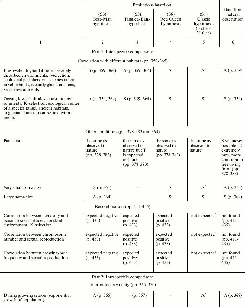
1 Because of a smaller interspecific competition.
2 Because of a greater DS.
3 Because of a greater interspecific competition.
4 Because of a smaller DS.
5 As DS is likely to be small during the parasitic phase and
great during the free-living phase.
6 As there is likely no related DS difference.
7 There is no reason to suppose a greater DS.
8 With an abrupt change of environment conditions a greater
DS is likely.
Notes: S = sexual; A = asexual; – no
prediction; DS = disadvantage of sex; T. = thelytoky (a rare
type of parthenogenesis in which females are produced from unfertilized
eggs).
This section has the same name as Chapter 4 in Bell’s book [5]. It also has similar aims; similar methods; predictions for the Best-Man, Tangled-Bank, and Red Queen hypotheses; and references to data from natural observations. The predictions in Table 3 for S3, S5, and S6 hypotheses are identical to those expounded by Bell; however, in situations where there is an absence in Bell’s opinion, a prediction has been proposed and a note has been added to provide an explanation.
The predictions of the “classic” hypothesis (S1) may be formulated by using one simple criterion: as the theory and the simulation model show, sex is always advantageous except in small and isolated populations and when the DS is important (for example, in severely disturbed environments, with r-selection, and in phases of exponential growth of population). Moreover, because the DS does not exist in the context of recombination, there is no correlation expected between certain phenomena of recombination (achiasmy, chromosome number, and crossing-over frequency) and amphimixis or parthenogenesis.
In various cases, the predictions of the “classic” hypothesis and those of other hypotheses coincide, although the motivations are different (for example, predictions of the “classic” hypothesis and those of the Red Queen for “Correlation with different habitats”).
A noteworthy result is the strong correspondence between predictions of the “classic” hypothesis and data from natural observation.
The failure of the Best-Man hypothesis (12 differences in Table 3) is remarkable, and Bell’s negative opinion on this theory [5] must be shared.
For the Tangled-Bank and the Red Queen hypotheses, there are the incorrect predictions regarding correlations between certain recombination phenomena and amphimixis or parthenogenesis (“Amphimixis is to parthenogenesis as high rates of recombination are to low; the correlates of low levels of recombination will therefore be the same as the correlates of parthenogenesis” [5]). This contradiction is described in more detail by Bell in Chapter 5.2 [5]. In contrast, because for phenomena such as achiasmy, the crossing-over frequency and the number of chromosomes DS cannot exist, a correlation between these phenomena and parthenogenesis is not predicted by the “classic” hypothesis, which is in accordance with data from natural observation [5].
Moreover, for the Tangled-Bank hypothesis, the prediction for parasitism is not completely adequate, as described by Bell [5].
Regarding other theories that are not considered in Table 3:
S2) Muller’s Ratchet hypothesis – This hypothesis could only justify sex for small populations: “Muller’s ratchet operates only in small or asexual populations … harmful mutations are unlikely to become fixed in sexual populations unless the effective population size is very small” [29]. Therefore, this theory, which is not contradicted by the results reported in this paper, could integrate the “classic” theory;
S4) Hitch-hiker hypothesis – An R+ gene could be described as a gene that is advantageous because it hitchhikes favorable genes that are better spread by its action. The hitch-hiker hypothesis could, therefore, be defined as a different and indirect way of expounding the “classic” theory;
S7) Historical hypothesis – This theory, which does not justify the existence of sex, is refuted by the evidence that sexual and asexual reproduction are influenced by many conditions. However, there is value in considering it not as a theory explaining sex but as an inertial factor that restrains an easy passage from sexual to asexual reproduction, or vice versa;
S8-S10) These hypotheses make no prediction.
Williams proclaimed ([3], p. 14): “…the unlikelihood of anyone ever finding a sufficiently powerful advantage in sexual reproduction with broadly applicable models that use only such general properties as mutation rates, population sizes, selection coefficients, etc.”, and Ridley wrote ([6], p. 29): “I asked John Maynard Smith, one of the first people to pose the question ‘Why sex?’, whether he still thought some new explanation was needed. ‘No. We have the answers. We cannot agree on them, that is all’”.
Perhaps, now Williams’ unlikelihood is a likelihood and the uncertainty of Maynard Smith has been solved. Based on theoretical arguments, the advantage of sex is rationally explained by the “classic” theory in terms of individual selection and by the use of only the “general properties…”, which Williams considered necessary [3]. Moreover, if we consider the DS, it is possible to formulate predictions about the trends of the diffusion of sexuality in nature and to confirm those trends using evidence from natural observations.
Muller’s Ratchet hypothesis, if confirmed, could reinforce and integrate the “classic” theory in the context of small populations. The historical hypothesis deserves attention as an inertial factor in the prediction of trends of the diffusion of sex and related phenomena.
The concept that biotic factors – which often determine oscillating s values – may be quantitatively more important than physical factors in terms of the selective forces that determine evolution (Red Queen concept), the pivotal idea at the root of the Red Queen hypothesis, is not contradictory to the “classic” theory, although it is insufficient in and of itself to explain sex, and it should be considered as an argument that reinforces the “classic” hypothesis.
The “pluralist approach to sex and recombination” [61] seems to be the correct solution to justify sex, but with the condition that the “classic” theory is the trunk with the main branches and some of the other theories complete the tree.
AGING
About aging, here defined as “increasing mortality with increasing chronological age in populations in the wild” [91], there are many theories [92-95], which can primarily be classified in two broad groups based on opposing paradigms:
– the first (“old paradigm”) interprets aging as the cumulative and progressive effect of many damaging factors that are insufficiently opposed by natural selection;
– the second (“new paradigm”) explains aging as a physiological function that is determined by natural selection in terms of supra-individual selection, but is opposed by individual selection.
Within the old paradigm, there are the following hypotheses:
O1) Cessation of somatic growth hypothesis. For this old theory, when the growth shows no limit, as in many lower vertebrates, the organism is always young and there is no aging. On the contrary, for species with a fixed growth, aging begins when the formation of new tissues ends [96-101].
O2) Damage accumulation hypothesis. This is a vast group of old and new theories that explain aging as being caused by the accumulation of various types of damage (“wear and tear”; deteriorations in cell colloids; degeneration of nervous or endocrine or vascular or connective tissues; toxic metabolites; damaging substances produced by gut bacteria; cosmic rays [92]; chemical damage due to DNA transcription errors [94]; and oxidative effects by free radicals on the whole body [102-105], on the DNA [94, 106], or on the mitochondria [107-110]).
O3) Mutation accumulation hypothesis. Aging is caused by many noxious genes that are insufficiently removed by natural selection because they manifest their actions late in life [111-115].
O4) Antagonistic pleiotropy hypothesis. Hypothetical pleiotropic genes, which are advantageous in younger ages and disadvantageous in older ages, are insufficiently eliminated by natural selection and cause a progressive decline in fitness [116, 117].
O5) Disposable soma hypothesis. It is assumed that the organism has limited resources, which are not well defined. Therefore, natural selection must divide them between the necessities of reproductive capacity and those of the maintenance systems, and the maintenance at older ages is sacrificed [118, 119].
O6) Quasi-programmed aging hypothesis [120]. This theory is a variation of the preceding hypothesis: “nature blindly selects for short-term benefits of robust developmental growth … aging is a wasteful and aimless continuation of developmental growth” [121].
O7) Historical hypothesis. In an analogy with the historical hypothesis for sex, a species could be more or less precociously aging, or even non-aging, if it belongs to a group of species, or to a phylum, where there is the same condition [122].
The following hypotheses are within the new paradigm:
N1) Aging as phenoptotic phenomenon. Aging appears to be under genetic determination and modulation, which means it must somehow be adaptive [123-126]. Aging is a particular type of a well-known group of phenomena [127], for which the neologism “phenoptosis” was coined [123], which defines the cases when an individual sacrifices itself, or its siblings, obligatorily or potentially, by mechanisms that are favored by natural selection at a supra-individual level [76, 123, 128].
N2) Aging is useful because it frees space for the next generation. Wallace, the coauthor of the first paper on evolution by natural selection, proposed that aging was favored by selection because predeceasing individuals do not compete with their offspring [129, 130]. Likewise, Weismann suggested (without any evidence) that aging is favored by evolution as the death of old individuals frees space for the next generation and that this was useful for accelerating evolution [17]; however, he later repudiated this idea [131, 132].
N3) Aging as increasing evolvability factor hypothesis. Following Weismann’s suggestion, aging is considered as favored by natural selection because it increases the speed and so the potentiality of evolution, or evolvability [133, 134].
N4) Red Queen hypothesis for aging. A proposed explanation for aging is that it would limit the spread of diseases caused by other living beings, an idea that is analogous to Red Queen hypothesis for sex [135], which is popular, but which appears to be untenable as shown by the simulation model and the evidence presented in the preceding section.
N5) Aging as caused by mitochondrial oxidative substances hypothesis. Mitochondrial reactive oxygen species (ROS) are thought to be the pivotal cause of aging, which is explained as a phenomenon that is favored by natural selection [130, 136, 137].
N6) “Chronomeres” and “printomeres” hypothesis. Hypothetical “chronomeres” and “printomeres” have been proposed as pivotal parts of programmed aging mechanisms [138, 139].
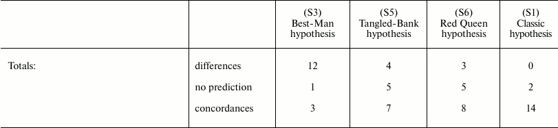
N7) Aging as an accelerating factor of evolution hypothesis. In 1961, Leopold, a botanist, again posed Weismann’s suggestion that aging accelerates the generation turnover and therefore favors evolution: “… in plants senescence is a catalyst for evolutionary adaptability” [140]. In 1983 and later, starting from the observation that an increase in the advantage (S) of a gene or an equivalent reduction of the mean duration of life (ML) have the same effect on the spread of a gene within a species (Fig. 9), the advantage of aging in spatially structured populations and in terms of kin selection was proposed [91, 141-145]. An analogous idea of the advantage of aging in spatially structured populations was later proposed using complex models [146-148]. However, the first model is much simpler and easier to understand. That model maintains that a gene C that determines a shorter ML is favored when:
n
Σ [r Sx (1/MLC – 1)] > S′, (16)
x = 1
where MLC = shorter ML of the individuals with C (while the individuals with the neutral allele C′ have MLC’ = 1); Sx = advantage of an x allele that is spreading within the species; m = number of alleles that are spreading within the species; r = relationship coefficient between the individual that dies by action of C and the substituting individual; S' = advantage of the greater ML of the individuals with the neutral allele C′.
Fig. 9. The figure on the left depicts the spread of gene C according to the variation of S, if ML is constant. The figure on the right depicts the spread of gene C according to the variation of ML, if S is constant. The simulation programs for Figs. 8 and 9 are available in the supplementary materials (see Supplement A to this paper on the site of the journal (http://protein.bio.msu.ru/biokhimiya)).
If the m alleles that are spreading within the species have a mean advantage of Sm, the formula (16) becomes:
m r Sm (1/MLC – 1) > S′, (17)
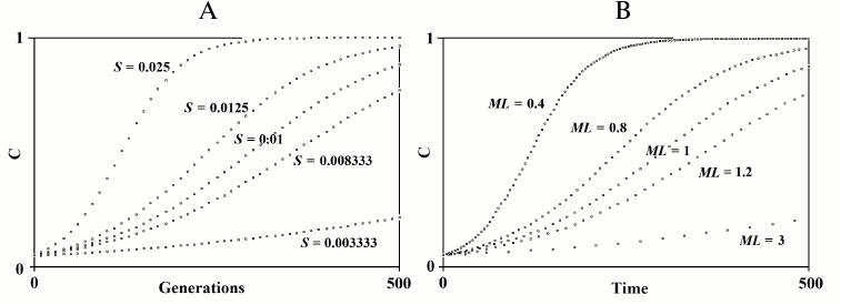
which has been used for Fig. 10.
Fig. 10. The spread or elimination of gene C that determines a reduced ML (MLC = 0.7). The value of C at generation 0 is equal to 0.1; Sm = 0.01; m = 600; S′ = 0.2. The values of r are indicated near each curve.
If C is a harmful gene (S < 0) instead of a favorable gene (S > 0), the same mechanism illustrated by formulas (16) and (17) causes a quicker elimination of C.
It is necessary to highlight that formulas (16) and (17) are equivalent to formula (10) used in the original work [91]:
r S (1/VC – 1) > S′, that is, r S (1/MLC – 1) > S′,
where it was “hypothesized S » S′, since S sums up the advantages of the m genes that are spreading within the species”. By disregarding this essential specification, which is now included in the formulas, the model has been wrongly considered as unlikely [149].
It is possible to highlight some common predictions for the hypotheses of the new paradigm: (i) possible existence of non-aging species; (ii) in the comparison among different species, an inverse relationship between extrinsic mortality and ML reduction caused by senescence (Ricklefs’ Ps, or proportion of senescent deaths [150]); and (iii) existence of specific, genetically determined and modulated, mechanisms that cause aging [143].
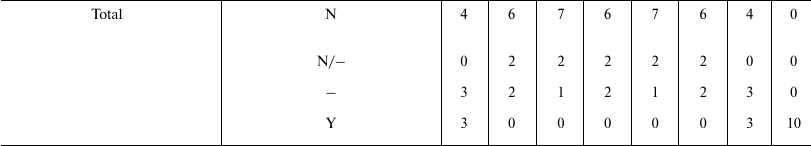
The arguments and the evidence that are in support of or against the old and the new paradigm have been discussed in another publication [95] and, for brevity, will not be repeated here. However, considering that work and adding the evaluation of the Historical hypothesis (O7), it is easily possible to organize Table 4 to show the correlations of the predictions of various hypotheses (O1-O7, N7) with empirical data or theoretical arguments. The other hypotheses are not considered in the table for the following reasons:
N1) Aging as phenoptotic phenomenon – is the main concept of the new paradigm, but is not a specific hypothesis;
N2) Aging is useful because it frees space for the next generation – may be considered an old and not a well-defined formulation of N7;
N3) Aging as increasing evolvability factor hypothesis. If aging accelerates the turnover of generations, this would increase the speed and the potentiality of evolution, that is, the evolvability. However, the proposed effect of aging should not be interpreted as the cause of it. For each function, it is correct to search for its meaning (teleonomy), but it is wrong to attribute a finalistic aim to this meaning (teleology). In other words, N3 should be considered a very important comment on the effects of aging and not a hypothesis about the evolutionary cause of aging;
N4 (Red Queen hypothesis for aging), N5 (Aging as caused by mitochondrial oxidative substances hypothesis), and N6 (“Chronomeres” and “printomeres” hypothesis) do not appear to give specific predictions that can be tested.
Table 4 shows that the predictions of N7 appear to be in total concordance with empirical data and theoretical arguments, while all the other hypotheses have not been proven true. Only the old Cessation of somatic growth hypothesis (O1) and the Historical hypothesis (O7) show a partial match with empirical data, and appear less contradicted by empirical data than the three theories (O2, O3, and O4) currently presented as the solid scientific explanation of aging.
Table 4. Correlations between empirical data
or theoretical arguments and the predictions of various hypotheses
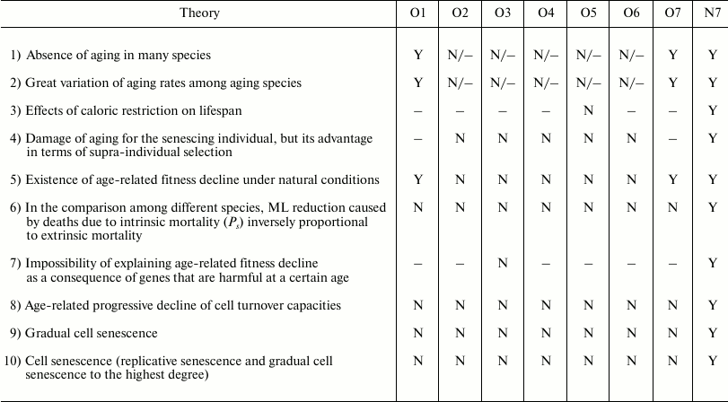
Notes: O1 = Cessation of somatic growth h.; O2 = Damage
accumulation h.; O3 = Mutation accumulation h.; O4
= Antagonistic pleiotropy h.; O5 = Disposable
soma h.; O6 = Quasi-programmed ageing h.; O7 =
Historical h.; N7 = Aging as accelerating factor of
evolution h.; N = not explained or predicted by the hypothesis
or in contrast with its predictions; – = irrelevant for the
purpose of accepting or rejecting the hypothesis; Y = predicted by the
hypothesis or compatible with it.
Comparison between sex and aging. Despite the large differences between sex and aging, there are several similarities that are worth highlighting.
Neither phenomena are favored by natural selection in populations that are numerically unlimited. Similarly, in conditions where there is high mortality and the need for rapid reproduction (mostly definable as conditions of r-selection), the disadvantages that are inherent to each of the two phenomena are greater. Therefore, species that reproduce asexually and species that do not age are predicted and exist.
Regarding sex, there are species that may alternate sexual and asexual phases, and the second alternative is preferred in r-selection conditions. For aging, there are not species with similar alternation of phases; however, under particular conditions (for example, caloric restriction), individuals of aging species appear to slow the aging process [151-157], a phenomenon that is incompatible with the theories that interpret aging as due to the action of damaging factors that are more or less effectively opposed.
To understand the evolutionary dynamic of both sex and aging, an analysis in terms of supra-individual selection is required.
Both phenomena increase the evolutionary potential of a species, that is, the evolvability. However, this is accomplished by two different mechanisms: sex accelerates the achievement of the best genetic combinations, while aging accelerates the spreading of favorable genes and the elimination of harmful genes. In any case, the greater evolvability must not be described as the factor that determines the evolution of the two phenomena: a greater evolvability is the effect and not the cause of the supra-individual selective mechanisms, which at each generation favor the genes determining sex or aging.
Regarding aging and sex as phenoptotic phenomena, there are the following conclusions:
– aging is a type of obligatory phenoptosis. It is a particular type of phenoptosis with a slow and progressive fitness decline and is therefore defined as “slow phenoptosis” [158];
– in general, sex does not imply obligatory death, but reduces the fitness as a consequence of the dangers caused by partner search, courtship, and mating. Most of the reduction in fitness is connected not so much to the sex itself, but to sexual differentiation. In some cases, sexual differentiation involves the sacrifice of one of the partners at the time of mating, after mating, or at the time of reproduction. Therefore, in general, sex can be classified as optional phenoptosis, although there are cases of obligatory phenoptosis.
The similarities and differences between sex and aging are summarized in Table 5.
Table 5. Similarities and differences
between sex and aging
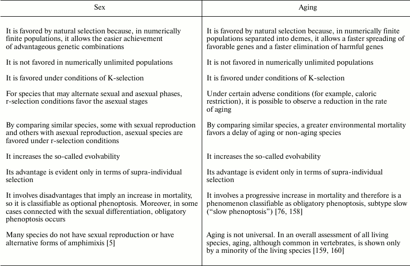
Both sex and aging are sometimes described as biological mysteries regarding their evolutionary justification.
However, if we analyze both phenomena in terms of supra-individual selection, a type of analysis that is absolutely necessary for any phenoptotic phenomenon, the advantages and disadvantages of the two phenomena become much clearer. The analysis of their advantages (in particular, in terms of supra-individual selection), together with the analysis of their disadvantages (in particular, at the individual level), may enable predictions about the conditions under which each of the two phenomena is favored or opposed by natural selection. These predictions, in the general evaluations of this review, appear to be fully supported by empirical evidence.
Another element that derives from the analysis in terms of supra-individual selection is that the cases of individual sacrifice (that is, the cases of phenoptosis), in their various forms for sex or aging (obligatory and slow, optional, obligatory and rapid), appear to be normal phenomena rather than anomalies that require explanations as strange exceptions.
REFERENCES
1.Pianka, E. R. (1970) On r- and K-selection, Am.
Nat., 104, 592-597.
2.Ghiselin, M. T. (1974) The Economy of Nature and
the Evolution of Sex, University of California Press, Berkeley.
3.Williams, G. C. (1975) Sex and Evolution,
Princeton University Press, Princeton.
4.Maynard Smith, J. (1978) The Evolution of
Sex, Cambridge University Press, Cambridge.
5.Bell, G. (1982) The Masterpiece of Nature. The
Evolution and Genetics of Sexuality, Croom Helm, London.
6.Ridley, M. (1993) The Red Queen. Sex and the
Evolution of Human Nature, Penguin Books, London.
7.Barton, N. H., and Charlesworth, B. (1998) Why sex
and recombination? Science, 281, 1986-1990.
8.Agrawal, A. F. (2006) Evolution of sex: why do
organisms shuffle their genotypes? Curr. Biol., 16,
R696-R704.
9.Hadany, L., and Comeron, J. M. (2008) Why are sex
and recombination so common? Ann. N. Y. Acad. Sci., 1133,
26-43.
10.Barton, N. H. (2009) Why sex and recombination?
Cold Spring Harb. Symp. Quant. Biol., 74, 187-195.
11.Otto, S. P. (2009) The evolutionary enigma of
sex, Am. Nat., 174, S1-S14.
12.Hartfield, M., and Keightley, P. D. (2012)
Current hypotheses for the evolution of sex and recombination,
Integr. Zool., 7, 192-209.
13.McDonald, M. J., Rice, D. P., and Desai, M. M.
(2016) Sex speeds adaptation by altering the dynamics of molecular
evolution, Nature, 531, 233-236.
14.Sharp, N. P., and Otto, S. P. (2016) Evolution of
sex: using experimental genomics to select among competing theories,
Bioessays, 38, 751-757.
15.Lewis-Pye, A. E., and Montalban, A. (2017) Sex
versus asex: an analysis of the role of variance conversion, Theor.
Popul. Biol., 114, 128-135.
16.Ho, E. K. H., and Agrawal, A. F. (2017) Aging
asexual lineages and the evolutionary maintenance of sex,
Evolution, doi: 10.1111/evo.13260.
17.Weismann, A. (1889) Essays upon Heredity and
Kindred Biological Problems, Translated by Poulton, E. B.,
Schonland, S., and Shipley, A. E., Clarendon Press, Oxford.
18.Guenther, C. (1906) Darwinism and the Problems
of Life. A Study of Familiar Animal Life, Translated by McCabe, J.
A., Owen, London.
19.Fisher, R. A. (1930) The Genetical Theory of
Natural Selection, Oxford University Press, Oxford.
20.Muller, H. J. (1932) Some genetic aspects of sex,
Am. Nat., 66, 118-138.
21.Muller, H. J. (1958) Evolution by mutation,
Bull. Am. Math. Soc., 64, 137-160.
22.Muller, H. J. (1964) The relation of
recombination to mutational advance, Mutat. Res., 1,
2-9.
23.Crow, J. F., and Kimura, M. (1965) Evolution in
sexual and asexual populations, Am. Nat., 99,
439-450.
24.Maynard Smith, J. (1968) Evolution in sexual and
asexual populations, Am. Nat., 102, 469-473.
25.Felsenstein, J. (1974) The evolutionary advantage
of recombination, Genetics, 78, 737-756.
26.Crow, J. F., and Kimura, M. (1969) Evolution in
sexual and asexual populations: a reply, Am. Nat., 103,
89-91.
27.Butcher, D. (1995) Muller’s ratchet,
epistasis and mutation effects, Genetics, 141,
431-437.
28.Gordo, I., and Charlesworth, B. (2000) The
degeneration of asexual haploid populations and the speed of
Muller’s ratchet, Genetics, 154, 1379-1387.
29.Keightley, P. D., and Otto, S. P. (2006)
Interference among deleterious mutations favors sex and recombination
in finite populations, Nature, 443, 89-92.
30.Gordo, I., and Campos, P. R. (2008) Sex and
deleterious mutations, Genetics, 179, 621-626.
31.Wardlaw, A. M., and Agrawal, A. F. (2012)
Temporal variation in selection accelerates mutational decay by
Muller’s ratchet, Genetics, 191, 907-916.
32.Williams, G. C. (1966) Adaptation and Natural
Selection. A Critique of Some Current Evolutionary Thought,
Princeton University Press, Princeton.
33.Emlen, J. M. (1973) Ecology: An Evolutionary
Approach, Addison-Wesley, Reading.
34.Treisman, M. (1976) The evolution of sexual
reproduction: a model which assumes individual selection, J. Theor.
Biol., 60, 421-431.
35.Dacks, J., and Roger, A. J. (1999) The first
sexual lineage and the relevance of facultative sex, J. Mol.
Evol., 48, 779-783.
36.Hill, W. G., and Robertson, A. (1966) The effect
of linkage on limits to artificial selection, Genet. Res.,
8, 269-294.
37.Case, T. J., and Taper M. L. (1986) On the
coexistence and coevolution of asexual and sexual competitors,
Evolution, 40, 366-387.
38.Burt, A., and Bell, G. (1987) Mammalian chiasma
frequencies as a test of two theories of recombination, Nature,
326, 803-805.
39.Doncaster, C. P., Pound, G. E., and Cox, S. J.
(2000) The ecological cost of sex, Nature, 404,
281-285.
40.Song, Y., Drossel, B., and Scheu, S. (2011)
Tangled Bank dismissed too early, Oikos, 120,
1601-1607.
41.Van Valen, L. (1973) A new evolutionary law,
Evol. Theory, 1, 1-30.
42.Hamilton, W. D. (1975) Gamblers since life began:
barnacles, aphids, elms, Quart. Rev. Biol., 50,
175-180.
43.Levin, D. A. (1975) Pest pressure and
recombination systems in plants, Am. Nat., 109,
437-451.
44.Charlesworth, B. (1976) Recombination
modification in a fluctuating environment, Genetics, 83,
181-195.
45.Glesener, R. R., and Tilman, D. (1978) Sexuality
and the components of environmental uncertainty: clues from geographic
parthenogenesis in terrestrial animals, Am. Nat., 112,
659-673.
46.Glesener, R. R. (1979) Recombination in a
simulated predator–prey interaction, Am. Zool., 19,
763-771.
47.Bell, G., and Maynard Smith, J. (1987) Short-term
selection for recombination among mutually antagonistic species,
Nature, 328, 66-68.
48.Peters, A. D., and Lively, C. M. (1999) The red
queen and fluctuating epistasis: a population genetic analysis of
antagonistic coevolution, Am. Nat., 154, 393-405.
49.Peters, A. D., and Lively, C. M. (2007) Short-
and long-term benefits and detriments to recombination under
antagonistic coevolution, J. Evolution. Biol., 20,
1206-1217.
50.Otto, S. P., and Nuismer, S. L. (2004) Species
interactions and the evolution of sex, Science, 304,
1018-1020.
51.Kouyos, R. D., Salathe, M., and Bonhoeffer, S.
(2007) The Red Queen and the persistence of linkage-disequilibrium
oscillations in finite and infinite populations, BMC Evol.
Biol., 7, 211.
52.Salathe, M., Kouyos, R. D., and Bonhoeffer, S.
(2008) The state of affairs in the kingdom of the Red Queen, Trends
Ecol. Evol., 23, 439-445.
53.Liow, L. H., Van Valen, L., and Stenseth, N. C.
(2011) Red Queen: from populations to taxa and communities, Trends
Ecol. Evol., 26, 349-358.
54.Brockhurst, M. A., Chapman, T., King, K. C.,
Mank, J. E., Paterson, S., and Hurst, G. D. (2014) Running with the Red
Queen: the role of biotic conflicts in evolution, Proc. Biol.
Sci., 281, pii: 20141382.
55.Voje, K. L., Holen, O. H., Liow, L. H., and
Stenseth, N. C. (2015) The role of biotic forces in driving
macroevolution: beyond the Red Queen, Proc. Biol. Sci.,
282, 20150186.
56.Stanley, S. M. (1978) Clades versus clones in
evolution: why we have sex? Science, 190, 382-383.
57.Kondrashov, A. S. (1984) Deleterious mutations as
an evolutionary factor. I. The advantage of recombination, Genet.
Res., 44, 199-217.
58.Charlesworth, B. (1990) Mutation selection
balance and the evolutionary advantage of sex and recombination,
Genet. Res., 55, 199-221.
59.Barton, N. H. (1995) A general model for the
evolution of recombination, Genet. Res., 65, 123-144.
60.Otto, S. P., and Feldman, M. W. (1997)
Deleterious mutations, variable epistatic interactions, and the
evolution of recombination, Theor. Popul. Biol., 51,
134-147.
61.West, S. A., Lively, C. M., and Read, A. F.
(1999) A pluralist approach to sex and recombination, J. Evol.
Biol., 12, 1003-1012.
62.Kondrashov, A. S. (1993) Classification of
hypotheses on the advantage of amphimixis, J. Hered., 84,
372-387.
63.Kondrashov, A. S., and Yampolsky, L. Y. (1996)
Evolution of amphimixis and recombination under fluctuating selection
in one and many traits, Genet. Res., 68, 165-173.
64.Burger, R. (1999) Evolution of genetic
variability and the advantage of sex and recombination in changing
environments, Genetics, 153, 1055-1069.
65.Palsson, S. (2002) Selection on a modifier of
recombination rate due to linked deleterious mutations, J.
Hered., 93, 22-26.
66.Iles, M. M., Walters, K., and Cannings, C. (2003)
Recombination can evolve in large finite populations given selection on
sufficient loci, Genetics, 165, 2249-2258.
67.Barton, N. H., and Otto, S. P. (2005) Evolution
of recombination due to random drift, Genetics, 169,
2353-2370.
68.Martin, G., Otto, S. P., and Lenormand, T. (2006)
Selection for recombination in structured populations, Genetics,
172, 593-609.
69.Tannenbaum, E. (2008) Comparison of three
replication strategies in complex multicellular organisms: asexual
replication, sexual replication with identical gametes, and sexual
replication with distinct sperm and egg gametes, Phys. Rev. E Stat.
Nonlin. Soft. Matter Phys., 77, 011915.
70.Otto, S. P., and Lenormand, T. (2002) Resolving
the paradox of sex and recombination, Nat. Rev. Genet.,
3, 252-261.
71.Felsenstein, J., and Yokoyama, S. (1976) The
evolutionary advantage of recombination, II. Individual selection for
recombination, Genetics, 83, 845-859.
72.Felsenstein, J. (1965) The effect of linkage on
directional selection, Genetics, 52, 349-363.
73.Eshel, I., and Feldman, M. W. (1970) On the
evolutionary effect of recombination, Theor. Pop. Biol.,
1, 88-100.
74.Karlin, S. (1973) Sex and infinity; a
mathematical analysis of the advantages and disadvantages of
recombination, in The Mathematical Theory of the Dynamics of Natural
Populations (Bartlett, M. S., and Hiorns, R. W., eds.) Academic
Press, London.
75.Armitage, P., Matthews, J. N. S., and Berry, G.
(2001) Statistical Methods in Medical Research, Wiley-Blackwell,
New York.
76.Libertini, G. (2012) Classification of
phenoptotic phenomena, Biochemistry (Moscow), 77,
707-715.
77.Zuk, M. (2016) Mates with benefits: when and how
sexual cannibalism is adaptive, Curr. Biol., 26,
R1230-R1232.
78.Polis, G. A. (1981) The evolution and dynamics of
intraspecific predation, Ann. Rev. Ecol. Syst., 51,
225-251.
79.Foelix, R. A. (1982) Biology of Spiders,
Harvard University Press, Cambridge (USA).
80.Bilde, T., Tuni, C., Elsayed, R., Pekar, S., and
Toft, S. (2006) Death feigning in the face of sexual cannibalism,
Biol. Lett., 2, 23-25.
81.Fernandez-Montraveta, C., Gonzalez, J. M., and
Cuadrado, M. (2014) Male vulnerability explains the occurrence of
sexual cannibalism in a moderately sexually dimorphic wolf spider,
Behav. Processes, 105, 53-59.
82.Gerritson, J. (1980) Sex and parthenogenesis in
sparse populations, Am. Nat., 115, 718-742.
83.Maynard Smith, J. (1971) The origin and
maintenance of sex, in Group Selection (Williams, G. C., ed.)
Aldine-Atherton, Chicago.
84.Lehtonen, J., Jennions, M. D., and Kokko, H.
(2012) The many costs of sex, Trends Ecol. Evol., 27,
172-178.
85.Parker, G. A., Baker, R. R., and Smith, V. G. F.
(1972) The origin and evolution of gamete dimorphism and the
male-female phenomenon, J. Theor. Biol., 36, 529-553.
86.Bell, G. (1978) The evolution of anisogamy, J.
Theor. Biol., 73, 247-270.
87.Charlesworth, B. (1978) The population genetics
of anisogamy, J. Theor. Biol., 73, 347-357.
88.Zahavi, A. (1975) Mate selection – a
selection for a handicap, J. Theor. Biol., 53,
205-214.
89.Maynard Smith, J. (1976) Sexual selection and the
handicap principle, J. Theor. Biol., 57, 239-242.
90.Alan Grafen, A. (1990) Biological signals as
handicaps, J. Theor. Biol., 144, 517-546.
91.Libertini, G. (1988) An adaptive theory of the
increasing mortality with increasing chronological age in populations
in the wild, J. Theor. Biol., 132, 145-162.
92.Comfort, A. (1979) The Biology of
Senescence, Elsevier North Holland, New York.
93.Medvedev, Z. A. (1990) An attempt at a rational
classification of theories of ageing, Biol. Rev. Camb. Philos.
Soc., 65, 375-398.
94.Weinert, B. T., and Timiras, P. S. (2003) Invited
review: theories of aging, J. Appl. Physiol., 95,
1706-1716.
95.Libertini, G. (2015) Non-programmed versus
programmed aging paradigm, Curr. Aging Sci., 8,
56-68.
96.Minot, C. S. (1907) The problem of age, growth,
and death; a study of cytomorphosis, based on lectures at the Lowell
Institute, March 1907, London.
97.Carrel, A., and Ebeling, A. H. (1921)
Antagonistic growth principles of serum and their relation to old age,
J. Exp. Med., 38, 419-425.
98.Brody, S. (1924) The kinetics of senescence,
J. Gen. Physiol., 6, 245-257.
99.Bidder, G. P. (1932) Senescence, Br. Med.
J., 115, 5831-5850.
100.Lansing, A. I. (1948) Evidence for aging as a
consequence of growth cessation, Proc. Natl. Acad. Sci. USA,
34, 304-310.
101.Lansing, A. I. (1951) Some physiological
aspects of ageing, Physiol. Rev., 31, 274-284.
102.Harman, D. (1972) The biologic clock: the
mitochondria? J. Am. Geriatr. Soc., 20, 145-147.
103.Croteau, D. L., and Bohr, V. A. (1997) Repair
of oxidative damage to nuclear and mitochondrial DNA in mammalian
cells, J. Biol. Chem., 272, 25409-25412.
104.Beckman, K. B., and Ames, B. N. (1998) The free
radical theory of aging matures, Physiol. Rev., 78,
547-581.
105.Oliveira, B. F., Nogueira-Machado, J.-A., and
Chaves, M. M. (2010) The role of oxidative stress in the aging process,
Sci. World J., 10, 1121-1128.
106.Bohr, V. A., and Anson, R. M. (1995) DNA
damage, mutation and fine structure DNA repair in aging, Mutat.
Res., 338, 25-34.
107.Miquel, J., Economos, A. C., Fleming, J., and
Johnson, J. E., Jr. (1980) Mitochondrial role in cell aging, Exp.
Gerontol., 15, 575-591.
108.Trifunovic, A., Wredenberg, A., Falkenberg, M.,
Spelbrink, J. N., Rovio, A. T., Bruder, C. E., Bohlooly, Y. M., Gidlof,
S., Oldfors, A., Wibom, R., Tornell, J., Jacobs, H. T., and Larsson, N.
G. (2004) Premature ageing in mice expressing defective mitochondrial
DNA polymerase, Nature, 429, 417-423.
109.Balaban, R. S., Nemoto, S., and Finkel, T.
(2005) Mitochondria, oxidants, and aging, Cell, 120,
483-495.
110.Sanz, A., and Stefanatos, R. K. (2008) The
mitochondrial free radical theory of aging: a critical view, Curr.
Aging Sci., 1, 10-21.
111.Medawar, P. B. (1952) An Unsolved Problem in
Biology, H. K. Lewis, London. Reprinted in: Medawar, P. B. (1957)
The Uniqueness of the Individual, Methuen, London.
112.Hamilton, W. D. (1966) The moulding of
senescence by natural selection, J. Theor. Biol., 12,
12-45.
113.Edney, E. B., and Gill, R. W. (1968) Evolution
of senescence and specific longevity, Nature, 220,
281-282.
114.Mueller, L. D. (1987) Evolution of accelerated
senescence in laboratory populations of Drosophila, Proc.
Natl. Acad. Sci. USA, 84, 1974-1977.
115.Partridge, L., and Barton, N. H. (1993)
Optimality, mutation and the evolution of ageing, Nature,
362, 305-311.
116.Williams, G. C. (1957) Pleiotropy, natural
selection and the evolution of senescence, Evolution, 11,
398-411.
117.Rose, M. R. (1991) Evolutionary Biology of
Aging, Oxford University Press, New York.
118.Kirkwood, T. B. (1977) Evolution of ageing,
Nature, 270, 301-304.
119.Kirkwood, T. B., and Holliday, R. (1979) The
evolution of ageing and longevity, Proc. R. Soc. Lond. B Biol.
Sci., 205, 531-546.
120.Blagosklonny, M. V. (2006) Aging and
immortality: quasi-programmed senescence and its pharmacologic
inhibition, Cell Cycle, 5, 2087-2102.
121.Blagosklonny, M. V. (2013) MTOR-driven
quasi-programmed aging as a disposable soma theory: blind watchmaker
vs. intelligent designer, Cell Cycle, 12, 1842-1847.
122.De Magalhaes, J. P., and Toussaint, O. (2002)
The evolution of mammalian aging, Exp. Gerontol.,
37, 769-775.
123.Skulachev, V. P. (1997) Aging is a specific
biological function rather than the result of a disorder in complex
living systems: biochemical evidence in support of Weismann’s
hypothesis, Biochemistry (Moscow), 62, 1191-1195.
124.Bredesen, D. E. (2004) The non-existent aging
program: how does it work? Aging Cell, 3, 255-259.
125.Mitteldorf, J. (2004) Aging selected for its
own sake, Evol. Ecol. Res., 6, 1-17.
126.Longo, V. D., Mitteldorf, J., and Skulachev, V.
P. (2005) Programmed and altruistic ageing, Nat. Rev. Genet.,
6, 866-872.
127.Finch, C. E. (1990) Longevity, Senescence,
and the Genome, The University of Chicago Press, Chicago.
128.Skulachev, V. P. (1999) Phenoptosis: programmed
death of an organism, Biochemistry (Moscow), 64,
1418-1426.
129.Wallace, A. R. (1889) The action of natural
selection in producing old age, decay and death (A note by Wallace
written “some time between 1865 and 1870”) (Weismann, A.,
ed.).
130.Skulachev, V. P., and Longo, V. D. (2005) Aging
as a mitochondria-mediated atavistic program: can aging be switched
off? Ann. N.Y. Acad. Sci., 1057, 145-164.
131.Weismann, A. (1892) Essays Upon Heredity and
Kindred Biological Problems, Vol. II, Clarendon Press, Oxford.
132.Kirkwood, T. B., and Cremer, T. (1982)
Cytogerontology since 1881: a reappraisal of August Weismann and a
review of modern progress, Hum. Genet., 60, 101-121.
133.Goldsmith, T. C. (2004) Aging as an evolved
characteristic – Weismann’s theory reconsidered,
Med. Hypotheses, 62, 304-308.
134.Goldsmith, T. C. (2008) Aging, evolvability,
and the individual benefit requirement; medical implications of aging
theory controversies, J. Theor. Biol., 252, 764-768.
135.Mitteldorf, J., and Pepper, J. (2009)
Senescence as an adaptation to limit the spread of disease, J.
Theor. Biol., 260, 186-195.
136.Skulachev, V. P. (1999) Mitochondrial
physiology and pathology; concepts of programmed death of organelles,
cells and organisms, Mol. Aspects Med., 20, 139-184.
137.Skulachev, V. P. (2001) The programmed death
phenomena, aging, and the Samurai law of biology, Exp.
Gerontol., 36, 995-1024.
138.Olovnikov, A. M. (2003) The redusome hypothesis
of aging and the control of biological time during individual
development, Biochemistry (Moscow), 68, 2-33.
139.Olovnikov, A. M. (2015) Chronographic theory of
development, aging, and origin of cancer: role of chronomeres and
printomeres, Curr. Aging Sci., 8, 76-88.
140.Leopold, A. C. (1961) Senescence in plant
development, Science, 134, 1727-1732.
141.Libertini, G. (1983) Evolutionary
Arguments, Societa Editrice Napoletana, Naples (Italy), English
Edn., 2011, Evolutionary Arguments on Aging, Disease, and Other
Topics, Azinet Press, Crownsville MD.
142.Libertini, G. (2006) Evolutionary explanations
of the “actuarial senescence in the wild” and of the
“state of senility”, Sci. World J., 6,
1086-1108.
143.Libertini, G. (2008) Empirical evidence for
various evolutionary hypotheses on species demonstrating increasing
mortality with increasing chronological age in the wild, Sci. World
J., 8, 183-193.
144.Libertini, G. (2009) The role of
telomere–telomerase system in age-related fitness decline, a
tameable process, in Telomeres: Function, Shortening and
Lengthening (Mancini, L., ed.) Nova Science Publ., New York, pp.
77-132.
145.Libertini, G. (2013) Evidence for aging
theories from the study of a hunter-gatherer people (Ache of Paraguay),
Biochemistry (Moscow), 78, 1023-1032.
146.Travis, J. M. (2004) The evolution of
programmed death in a spatially structured population, J. Gerontol.
A Biol. Sci. Med. Sci., 59, 301-305.
147.Martins, A. C. (2011) Change and aging
senescence as an adaptation, PLoS One, 6, e24328.
148.Mitteldorf, J., and Martins, A. C. (2014)
Programmed life span in the context of evolvability, Am. Nat.,
184, 289-302.
149.Kowald, A., and Kirkwood, T. B. (2016) Can
aging be programmed? A critical literature review, Aging Cell,
doi: 10.1111/acel.12510.
150.Ricklefs, R. E. (1998) Evolutionary theories of
aging: confirmation of a fundamental prediction, with implications for
the genetic basis and evolution of life span, Am. Nat.,
152, 24-44.
151.Calabrese, E. J., and Baldwin, L. A. (1998)
Hormesis as a biological hypothesis, Environ. Health Perspect.,
106, 357-362.
152.Masoro, E. J. (2003) Subfield history: caloric
restriction, slowing aging, and extending life, Sci. Aging Knowledge
Environ., RE2.
153.Masoro, E. J. (2005) Overview of caloric
restriction and ageing, Mech. Ageing Dev., 126,
913-922.
154.Masoro, E. J. (2007) The role of hormesis in
life extension by dietary restriction, Interdiscip. Top.
Gerontol., 35, 1-17.
155.Calabrese, E. J. (2005) Toxicological
awakenings: the rebirth of hormesis as a central pillar of toxicology,
Toxicol. Appl. Pharmacol., 204, 1-8.
156.Ribaric, S. (2012) Diet and aging, Oxid.
Med. Cell Longev., 741468.
157.Lee, S. H., and Min, K. J. (2013) Caloric
restriction and its mimetics, BMB Rep., 46, 181-187.
158.Skulachev, V. P. (2002) Programmed death
phenomena: from organelle to organism, Ann. N.Y. Acad. Sci.,
959, 214-237.
159.Jones, O. R., Scheuerlein, A., Salguero-Gomez,
R., Camarda, C. G., Schaible, R., Casper, B. B., Dahlgren, J. P.,
Ehrlen, J., Garcia, M. B., Menges, E. S., Quintana-Ascencio, P. F.,
Caswell, H., Baudisch, A., and Vaupel, J. W. (2014) Diversity of ageing
across the tree of life, Nature, 505, 169-173.
160.Libertini, G., Rengo, G., and Ferrara, N.
(2017) Aging and aging theories, J. Geront. Geriatr., 1,
59-77.
Supplement A+B: Simulation Figs. S1-S12 and raw data of the simulations (PDF)
Simulation programs (ZIP)