The Informativeness of Coherence Analysis in EEG Studies
г A. P. Kulaichev.
source: Neuroscience and Behavioral Physiology, 41(3): 321-328, 2011
Abstract.
Numerous methodological and computational errors typical of coherence analysis
of EEG recordings are discussed. Comprehensive review of the fundamental
disadvantages of coherence functions shows that this measure cannot be
regarded as a reliable and effective indicator of the synchronicity of
EEG processes.
Keyworgs:
coherence, spectral analysis, EEG non-stationarity, amplitude modulation
The first application of mathematical methods into electroencephalography is traditionally associated with N. Viner, who proposed the use of correlation analysis in 1936, taking the EEG to be a stationary wave process. The intensive application of mathematical methods charac-terized the first stage in the development of computerized electrophysiology [6, pp. 20–32]. This was taken up by physiologists and the engineers working with them with great enthusiasm. However, professional mathematicians, who do not see any great scientific prestige from immersing themselves deeply in this field, generally restrict themselves to overall theoretical positions expressed in general terms. The introduction of mathematical methods by technical specialists led to the diffusion of a wide range of incorrect and even erroneous methods, viewpoints, and concepts among physiologists. In particular, the two fundamental dif-ferences between EEG signals and most other physical signals are not considered: a) fundamental non-stationarity; b) amplitude modulation at all frequency ranges. This applies to a particularly critical extent to coherence analysis, to which attention has been drawn previously [5].
Sources.
According to [7, p. 138], “Goodman first proposed the so-called coherence
function in 1960 [15] and studies reported in [14] its first use in the
analysis of brain bioelectrical activity.” On the one hand, studies in
[15] did not consider or mention coherence, while spectral analysis methods
had been developed long before this and were resumed in basic monographs
from well known authors such as Barlett (1955), Bendat (1958), Blackman
and Tewkey (1959), and others. On the other hand, the coherence for-mula
as applied to electrophysiology was introduced and commented on (without
source references) by one of the authors of [14] in later studies [17].
It should also be
noted that the extensive specialist literature on coherence has a number
of deficiencies. Thus, the coherence function for processes x(t) and y(t)
(some-times termed coherence squared) is usually stated as:
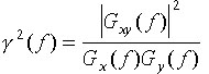 ,
(1)
,
(1)Mathematical definitions. Let there be two monoharmonic and centered processes with some frequency f:
We will use E[...] to indicate the operation of averag-ing for the ensemble for nonoverlapping epochs (Bartlett method). One possible averaging formula for calculating the square of the coherence will then be of the form:
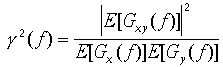 ,
(9)
,
(9) Coherence
in technical addenda. Methods for spectral
analysis were initially used for signals of physical origin and were only
later applied to EEG investigations. In technical addenda, coherence is
used as a particularly second-degree characteristic – only for evaluating
the significance of other cross-spectral characteristics and for defining
measures of the influence on them of noise and/or nonlinearity. Decreases
in coherence values can result from the following main causes [1, p. 179;
11. p. 271]:
1) presence of noncorrelating noises in signals
determining instability in the phase of the cross spectrum over time;
2) the presence of nonlinear relationships
between processes;
3) leakage of power determined by inadequate
frequency resolution, i.e., observation periods of insufficient duration;
4) the presence of time delays on transfer
of interactions between two pro-cesses commensurate with the observation
interval.
Small coherence values
can indicate the insignificance, at the frequency being addressed, of other
cross-spectral characteristics or can indicate the need to increase the
num-ber of averagings to eliminate the effects of noise.
The cardinal difference
is that signals of physical origin often truly have stationary harmonics
created by real sources: radio stations operating at their characteristic
frequency; errors in the geometry of the moving part of a mechanism inducing
vibration, etc. By recording the radio background at different locations
at the frequency of a given radio station, we will at any time point have
a fixed phase difference (determined by the distance of the measuringpoints
from the source). If there is radio noise at this frequency, then the cross-phase
of this harmonic will show some degree or other of change; coherence allows
this vari-ability to be evaluated and increases in the number of averagings
allow it to be decreased.
In the brain there
are actually no harmonic oscillators or anything producing stationary reflections
in the EEG. Arbitrarily dividing the frequency band into spectral lines
(defined by the duration of the analysis epoch), Fourier transformation
yields pseudoharmonics as a result of interference between a multiplicity
of uncontrolled and unknown factors, and these harmonics change from epoch
to epoch. This is reflected primarily on instantaneous autospectra, where
each harmonic does not have a smooth transition at the boundary of two
neighboring analysis epochs, but rather sharp, random jumps in amplitude,
and, consequently, in phase. These jumps are then reproduced in the cross-phase
of the two processes and hence in coherence values.
In summary, we can
conclude that the large and unique value that coherence has acquired in
EEG studies as compared with its background position in primary sources
is ungrounded. Coherence was developed to solve other tasks and is based
on other premises, so efforts should have been made to find and construct
more appropriate and reliable measures at the very beginning of its EEG
application.
The needs
of electrophysiology. In the physiology of higher nervous
activity, it is important to have reliable assessments of different aspects
of the synchronicity of EEG processes. When high synchronicity is present,
the presence of different types of physiological relationships between
processes can be proposed and verified: the effects of one process on the
other, the influence of a common source on both processes, and detection
of topographical patterns of highly synchronized relationships with the
aim of differentiating functional states, personal characteristics, normal
and pathological, the effects of drugs, etc.
The attraction of coherence for these purposes
appears largely to result from the repeatedly published and insufficiently
discussed proposition that coherence in a frequency
range is an analog of the Pearson correlation coefficient over a
time period [2, p. 112; 10, p. 342; 11, p. 270; 13, p. 36; 17, p. 172].
As will be shown twice, these propositions are quite far from reality.
Here, in particular, we will note that a) coherence (Equation (1)) can
relate only to the square of the correlation coefficient, which in practice
is extremely rarely used; b) unlike coherence, the range of values of the
correlation coefficient is from –1 to +1. Interpretation of coherence.
Equation (9) does not give a direct and clear informative interpretation
of coherence. We will therefore consider another acceptable version of
Equation (1) [6, p. 196], whose denominator is a transformation using Equation
(7):
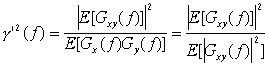 , (10)
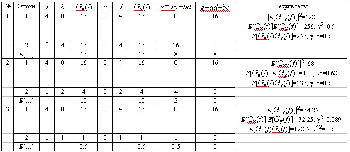
Thus, g2 coherence gives an increased assessment in relation to the extent of synchronicity of the processes, with a complex relationship with the extent of their amplitude variability. This coherence is fundamentally different from the correlation coefficient as a stable indicator of a linear relationship between two paired values which are not dependent on the ratio of the ranges of their values.TABLE 1. Relationship between Coherence and Amplitude-Phase Ratios of the Spectra of Two Monoharmonic Signals
Errors
in spectral analysis. One of the main
errors in discrete Fourier transformation (DFT) arises from leakage or
drainage of power from spectral peaks to neighboring
spectral lines. In technical addenda, this
is decreased by using a variety of correcting windows and this method has
been transported uncritically into electrophysiology.
However, studies reported in [6, p. 200] showed that windows have a double
effect on spectral peaks: they compress broad peaks but broaden well localized
peaks. Therefore it is more correct to calculate the mean and maximum amplitudes
of a spectrum after preliminary filtration of the signal in the range being
analyzed, which excludes leakage and modulating peaks from neighboring
ranges.
However, the leakage
effect depends on the ratio of the harmonic period and the analysis epoch
[6, p. 200]: there is no leakage when there is a whole number of harmonic
periods per analysis epoch and leakage is maximal when there is a half-integer
number of harmonic periods per analysis epoch. Furthermore, even in the
latter case, leakage decreases in inverse proportion to increases in distance
from the main peak. However, there is a further, not previously noted,
but important distortion to spectra, associated with the amplitude modulation
present in all EEG signals. This effect [6, p. 187] results in the appearance
of two symmetrical side peaks of 40% or more of the amplitude of the central
peak and separated from it by a number of spectral lines equal to the number
of signal modulation periods observed (this applies to monoharmonic signals,
and the situation with real EEG traces will be significantly more complex).
These two main errors
produce additional (to the abovenoted) random fluctuations in spectra,
which are par-ticularly clear visually when frequency resolution is high.
Phase spectra are more subject to these fluctuations than amplitude spectra.
 a)
a)
 b)
b)
 c)
c)
 d)
d)
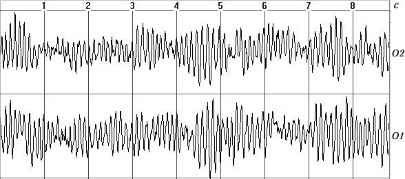
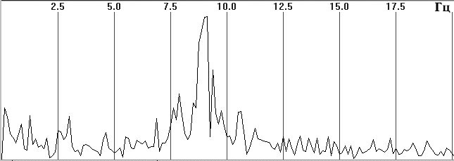
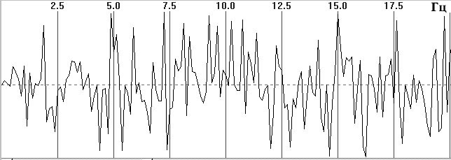
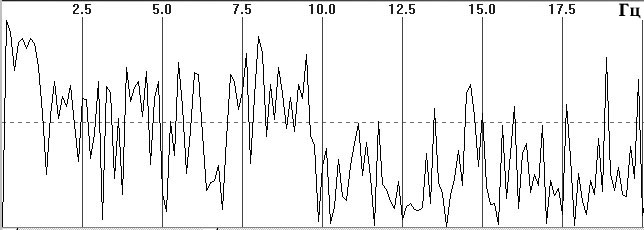
Fig. 1. Typical EEG spectra. a) Occipital EEG lead with a high alpha-rhythm
content (9-sec trace), sampling frequency 128 Hz, analog filters with bandpass
0.5–32 Hz, total trace duration 64 sec; b) amplitude cross-spectrum (one
8-sec epoch); c) phase cross-spectrum (one 8-sec trace); d) coherence spectrum
(average of 8 epochs).
Figure 1, a shows a small fragment of a typical and prolonged EEG trace with a high alpha-rhythm content in the two occipital leads. Figure 1, b shows the amplitude cross-spectrum between these two processes for an 8-sec analysis epoch, which reveals a high-amplitude peak at the fundamental frequency of the alpha rhythm, 9 Hz. The presence of low-amplitude random fluctuations throughout the frequency range should also be noted. Figure 1, c, d shows the phase cross-spectrum and the coherence spectrum, which are already completely dominated by random fluctuations and no clear frequency pattern can be discriminated. Figure 2 shows a plot of changes in cross-spectrum phase at the fundamental alpha-rhythm frequency of 9 Hz for 32 sequential epochs. This shows that the phase (whose stabil-ity significantly reflects coherence) shows random and large epoch-by-epoch variations over the wide range ±160°. This randomly fluctuating nature of oscillations in coher-ence and phase is typical of illustrations presented in phys-iology reports [8, pp. 68–82; 12, p. 29; 13, pp. 134–137, and others]. The situation with averaged coherence values is no better (see below).
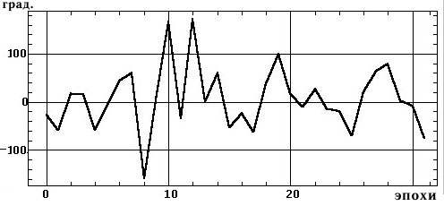
Fig. 2. Changes in cross-spectrum phase (Fig. 1, c) for the dominant
alpha-rhythm frequency of 9 Hz (Fig. 1, b) at 32 sequential 2-sec epochs
Sharp reductions in the accuracy of calculations
for small signal amplitudes should be noted, these being characteristic
of high-frequency ranges and due to the limited data element length resulting
from the integer-based representation of the output of analog-to-digital
converters – low-amplitude harmonics are represented by the least significant
bits. This affects first the accuracy of calculations of autospectrum and
cross-spectrum amplitudes and then, to a greater extent, coherence values.
This effect is a further source of error in coherence analysis.1 In this
regard we must not criticize modern ACD with high bit coding (up to 24-bit)
which use delta-sigma conversion; these ACD record all signals from the
surrounding space and particularly the high-amplitude network noise. After
its removal by digital filtration, the extracted EEG signal is generally
located in the 8–12 least significant bits.
Thus, coherence is extremely dependent
on random fluctuations resulting from fundamental instrument errors associated
with DFT and the properties of the EEG processes themselves. This also
has the result that coherence cannot be regarded as an informative measure
for evaluat-ing the levels of synchronicity of EEG processes. According
to the popular expression: anything can be extracted from Gaussian noise.
Dependence
on noise level. An important question,
ignored in the literature, is that of elucidating the relation-ship between
coherence and the levels of noise in the sig-nals being analyzed. We will
address this using a statistical modeling method, which is based on a very
simple concept. The instantaneous spectra X(f) and Y(f)
of monoharmonic processes x(t) and y(t) are
generated by geometrical summation of two components: a) a defined vector
of length r with a range of values r = 0-1 with a fixed phase
angle (for example, 0°), and b) a random vector of length 1 r with
a phase angle selected randomly in the range 0–360°. Each coherence value
is calculated by averaging 30 pairs of such instantaneous spectra and the
mean value is calculated using 1000 g2
values calculated in this way.an essentially linear relationship with noise,
i.e., 20–60%; 4) when signals contain more than 30–40% noise it becomes
difficult to claim a high level of synchronicity between EEG processes,
such that only g2
values of >0.7 are acceptable for this.
ntent in the narrow range over which the curve
shows an essentially linear relationship with noise, i.e., 20–60%; 4) when
signals contain more than 30–40% noise it becomes difficult to claim a
high level of synchronicity between EEG processes, such that only g2>0.7
are acceptable for this.
The relationship
between the mean value of g2
and the noise content in the signal (0–r)% is shown in Fig. 3, and
this plot leads to the following conclusions: 1) The Sshaped nature of
this relationship fundamentally distinguishes coherence from the correlation
coefficient, whose relationship with the noise level is essentially linear;
2) at noise levels exceeding 60%, the relationship is largely flattened,
so over this range g2
cannot serve as a measure of the noise content or the extent of desynchronization
of EEG processes; 3) g2
can only be a satisfactory indicator of noise content in the narrow range
over which the curve shows
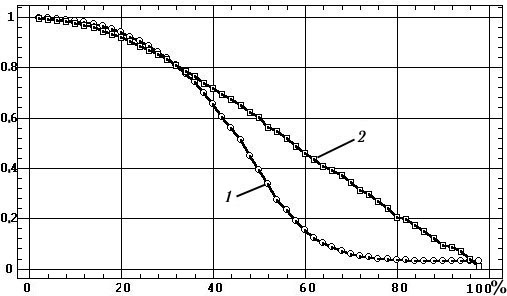
Fig. 3. Relationship between coherence values
(1) and correlation coefficients (2) and the proportion of noise in the
signal.
These conclusions
are supplemented by data reported in [1, p. 308] on the number of averagings
n required to obtain significant values of g2
with errors levels of less than ±0.1 depending on the true value of g2
(Table 2). As the non-stationarity of EEG processes over prolonged periods
of time has the result that the number of averagings available for coherence
calculations is generally no more than 10, it follows that only values
of g2>0.8
can be regarded as satisfactorily significant.
However, scientific
reports generally discuss experimental assessments of coherence in the
range 0.1–0.8 and use these to draw physiological conclusions. These conclusions
may therefore be extremely mediocre evaluations of the levels of synchronicity
of EEG processes.
Computer analyzers.
What situation applies to the various commercialized programs for coherence
calcula-tions? We asked several leading and senior EEG analyzer producers
(in Moscow, St. Petersburg, Taganrog, Ivanovo, Kharkov) about their algorithms
for calculation of coherence and received responses whose agreement was
far less than 100%.
Testing of a number of program bundles
using identical EEG traces showed (uniformity of testing was hindered by
the incompatibility of the programs in terms of loading traces in the international
EDF format) that the correspondence of coherence spectra applies only in
relation to their integral characteristics (one comparison example is shown
in Fig. 4): plots were monotonic or multipeak, had neighboring high or
low values at particular frequencies, and had approximate coincidence of
the frequency values of certain peaks. Other qualitative characteristics,
as well as quantitative evaluations, showed significant differences. This
would appear to result from the relationship between coherence values and
a multitude of parameters undeclared on the packaging and uncontrolled:
squared or nonsquared versions of the computations, the length of the analysis
epoch, the number of epochs averaged, the magnitude of the time shift between
epochs, the use of a correcting window, the type of final smoothing of
the coherence function, etc.
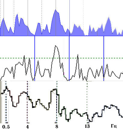
Fig. 4. Coherence spectra calculated using
three EEG analyzers, epoch length 4 sec, average of 16 epochs..
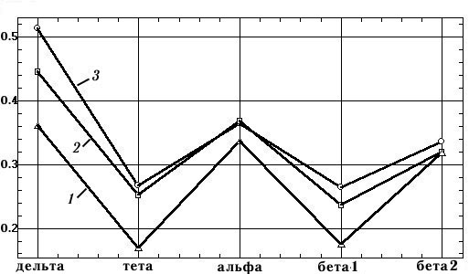
An example of the dependence of a coherence spectrum on the duration of the epochs being averaged and the correcting window is shown in Fig. 5. This clearly shows that the results are significantly different in terms of the positions, shapes, and amplitudes of the dominant peaks.
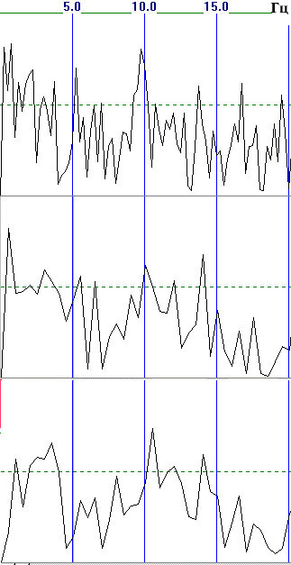
Figure 6 shows plots of the mean coherence values in standard frequency ranges calculated for the spectra of Fig. 5. The range of variation of coherence values is very large – amounting to 28–36% of the maximum value (in the delta, theta, and beta1 ranges). Thus, the mean coherence calculated using different values for the parameters are not comparable in quantitative terms. The variability increases even more when we calculate mean coherence for a group of subjects [8, pp. 71, 74], when most paired differences in coherence, on the background of large standard deviations, are statistically insignificant.
It should also be noted that recent years
have seen the increasing introduction of new spectral analysis methods
based on wavelets, which produce results even more fundamentally (both
quantitatively and qualitatively) different from the results obtained using
traditional DFT and, thus, from the whole assemblage of data accumulated
over many decades.
Thus, coherence analysis results obtained
using dif-ferent program bundles and with different values for the parameters
are poorly comparable in qualitative and quantitative terms, as are any
scientific conclusions based on these results.
Conclusions.
This multilateral analysis of the fundamental disadvantages of coherence
functions (identification of the influences of a multitude of uncontrolled
fandom factors, inapplicability to EEG analysis, dependence on a number
of adjusting factors, the nonlinearity of the dependence on the noise level,
dependence on phase and amplitude variability, the non-comparability of
the results obtained, etc.) indicates that this numerical characteristic
cannot, on the basis of metrological considerations, be supported as an
analytical tool in the current understanding of this term.
Alternatives.
Many investigators have in recent years recognized the stationary-segments
paradigm of EEG structure [3], such that various approaches can be applied
to EEG traces using relatively stationary segments with a criterion for
the synchronicity of the time dynamics of such structures. One potential
approach in this direction [4 and others] is based on segmentation for
areas of increased/decreased amplitude modulation of signals, with evaluation
of the synchronicity of two leads in terms of the proportion of coinciding
intersegment transitions (an algorithmic approach to this method is presented
in [6, pp. 227–230, 251–254]. Another approach consists of using Pearson
correlation coefficients to assess the synchronicity of EEG modulation
rhythms in a selected time period. Both of these methods have now been
verified and the results obtained using them demonstrate their applicability
to many probems and their potential.
REFERENCES
1. J. Bendat and A. Pirsol, Measurement and Analysis of Random Processes
[Russian translation], Mir, Moscow (1971).
2. G. Jenkins and D. Watts, Spectral Analysis and its Applications
[Russian translation], Mir, Moscow (1971).
3. A. Ya. Kaplan, “EEG nonstationarity: methodological and experimental
analysis,” Usp. Fiziol. Nauk., 29, No. 3, 35–55 (1998).
4. A. Ya. Kaplan, S. V. Borisov, S. L. Shishkin, and V. A. Ermolaev,
“Analysis of the segment structure of human EEG alpha activity,” Ros. Fiziol.
Zh., 4, 84–95 (2002).
5. A. P. Kulaichev, “Some methodological problems of EEG frequency
analysis,” Zh. Vyssh. Nerv. Deyat., 47, No. 5, 918–926 (1997).
6. A. P. Kulaichev, Computerized Electrophysiological and Functional
Diagnosis [in Russian], FORUM-INFRA-M, Moscow (2007).
7. M. N. Livanov, Temporospatial Organization of Potentials and
Systems Activity in the Brain [in Russian], Nauka, Moscow (1989).
8. M. N. Livanov, V. S. Rusinov, P. V. Simonov, M. V. Frolov, O.
M. Grin-del, G. N. Boldyreva, E. M. Vakar, V. G. Volkov, T. A. Maiorchik,
and N. E. Sviderskaya, Diagnosis and Prognosis of the Functional State
of the Brain [in Russian], Nauka, Moscow (1988).
9. S. L. Marple, Jr., Digital Spectral Analysis and its Applications
[Russian translation], Mir, Moscow (1990).
10. R. Otnes and L. Enoxon, Applied Analysis of Time Series [Russian
translation], Nauka, Moscow (1978).
11. R. B. Randall, Frequency Analysis, Bruel and Kjaer, Copenhagen
(1989).
12. V. S. Rusinov, O. M. Grindel, G. N. Boldyreva, and E. M. Vakar,
Biopotentials in the Human Brain [in Russian], Meditsina, Moscow (1987).
13. V. D. Trushch and A. V. Korinevskii, Computers in Neurophysio-logical
Studies [in Russian], Nauka, Moscow (1978).
14. W. R. Adey and D. O. Walter, “Application of phase detection
and averaging techniques in computer analysis of EEG records in the cat,”
Exper. Neurol., 7, 186–209 (1963).
15. N. R. Goodman, “Measuring amplitude and phase,” J. Franklin
Inst., 270, 437–450 (1960).
16. G. Nolte, O. Bai, L. Wheaton, Z. Mari, S. Vorbach, and M. Hallett,
“Identifying true brain interaction from EEG data using the imagi-nary
part of coherency,” Clin. Neurophysiol., 115, 2292–2307 (2004).
17. D. O. Walter, “Spectral analysis for electroencephalograms:
Mathe-matical determination of neurophysiological relationships from records
of limited duration,” Exper. Neurol., 8, 155–181 (1963).
![]()