COMPARSION OF REAL EEG REFERENCES
WITH AND WITHOUT ZERO POTENTIAL ACCORDING RESULTING TOPOGRATHY DIFFERENCIES
г
A.P. Kulaichev, 2016
citing:
Moscow University Biological Sciences Bulletin, 2016, Vol. 71, No. 3, pp.
145–150.
Abstract: The
problem to find an optimal EEG reference is the actual topic for discussion
over 60 years. We have studied topographical differences in averaged EEG
amplitudes in alpha domain recorded in 10–20 system during “eyes closed”
test. These differences appeared due to the use of 13 reference schemes:
top and bottom of the chin (Ch1, Ch2); nose (N); top and bottom of the
neck (Nc1, Nc2); upper back (Bc); united electrodes at the base of the
neck anteriorly and posteriorly (2Nc); united, ipsilateral, and individual
ear electrodes (A12, Sym, A1, A2); vertex (Cz); and averaged reference
(AR). Six experiments for each of the ten subjects were carried out with
grounded and ungrounded states of three distant basic references Ch2, Bc,
2Nc. Pairwise comparisons of topographic consistency of 13 reference schemes
were carried out on the proposed complex of three independent indicators
with evaluative criterion, followed by centroid-based clustering of the
reference schemes and its discriminant verification. As a result, we have
established: (1) that most coordinated topography is provided by the following
reference electrodes — A12, P1, P2, Sym; (2) reference electrodes A1, Sh2,
A2, Sh1, AR, Cz are characterized by individually varying topography, which
may lead to contradictory conclusions obtained when they are used; (3)
no significant reasons have been found for preferring the grounded (neutral)
states of reference electrodes, that makes the search for or mathematical
construct of an infinitely remote neutral reference electrode less important;
(4) numerous distortions of EEG topography by reference electrode standardization
technique (REST) raise serious doubts about its proclaimed advantages in
EEG studies.
Key
words: EEG, reference electrode, reference
at infinity, neutral reference, spectral analysis, cluster analysis, discriminant
analysis, topographical analysis, REST reference electrode standardization
technique..
1. Introduction
The history of EEG studies
ascends to 1875 when English surgeon Richard Caton have found the changes
of electric current on an open rabbit’s and monkey’s brain. Half a century
later in 1924 German neurologist Hans Berger [3] have recorded the electric
waves from a human scalp. He also introduced the term “electroencephalogram”
and revealed the EEG dependence on a number of functional states and some
nervous diseases. Later E. Adrian and B. Matthews [1] have revealed the
regular waves from 10 to 12 Hz which they introduced as “alpha rhythm”.
These works gave an impetus to development of EEG investigations during
next decades. The important standardization of EEG studies have took place
in 1958 when International Federation of Electroencephalography and Clinical
Neurophysiology approved 10-20% system of electrodes placement offered
by Canadian neurophysiologist Herbert Jasper [15]. However neither before
nor after no consensus was found on the location of the reference electrode,
which would be preferable for EEG recording on the scalp using monopolar
montage [5, 24, 25, 28, 31].
In the early 1950s,
summarization of the preceding discussion showed [29] that the use of earlobes
individually induced a decrease in EEG amplitude due to their proximity
to the temporal electrodes. The pathological activity in the temporal region
is reflected on the data from the ear electrodes, and this affects results
obtained from the other electrodes via the reference. The reference electrodes
on the nose and face are sensitive to artifacts from eye movement. The
placement of reference electrodes on the body leads to the appearance of
ECG and other artifacts. The positioning of electrodes at the base of the
neck anteriorly and posteriorly was proposed, which, when connected to
scalp, results in approximately the same voltage but of the opposite sign,
so this association provides unobtrusive secondary voltage.
Much later [31],
the use of the following references was discussed: the vertex (Cz), the
linked ear and linked mastoid electrodes, ipsilateral or contralateral
ears, nose tip, bipolar reference electrodes, the averaged reference (AR),
weighted AR, and the reference of source derivation. Each of them has its
advantages and disadvantages and can cause various distortions in the topographic
pattern of EEG potentials distribution. More distant references located
on the thumb, elbow, knee, shoulder, neck, chest, back, and nose are discussed
[10, 33]. However, prospects of discovering a potential close to zero or
the ideal reference electrode on the body at a large distance from the
neural sources have repeatedly been questioned [12, 16, 24].
In addition, in recent
years, mathematical methods of designing the inactive neutral reference
have appeared: the reference electrode standardization technique, REST
[27, 34], blind source separation, BSS [21], minimum power directionless
response, MPDR [11], current source density derivations, CSD [4, 9], robust
maximum-likelihood type estimator [20], spherical spline interpolation
methods [26] and others.. These methods continue to be modified and support
positive expectations [16], but they rather have the nominal and theoretical
value than the actual use and verification in practice.
Thus, this problem
is still far from a final solution, which determines the importance of
new approaches to the subject, especially with regard to the comparison
of actual physical reference electrodes.
In this work we studied
the topographical distinctions of EEG amplitude distribution over a scalp
caused by the use of different references schemes. Indeed, the topographic
relations are fundamentally important for inter-group comparisons in studies
of various functional states, pathologies, sexual, age, professional, ethnic,
regional and other distinctions. If two references vary greatly in obtained
scalp topography then EEG results will be incomparable [16]. For example,
if EEG amplitude at A electrode is greater compared to B electrode in chosen
reference scheme but in other scheme this ratio is opposite then resulting
physiological findings and clinical conclusions may be controversial. On
the other hand, as it follows from the above review, the use of stable
neutral reference should provide the correct values of EEG potentials as
well as the correct EEG topography.
2. Material and methods
In our experiments we
use the "closed eyes" state in a relaxed sitting position. Such a condition
exclude the appearance in the records an artifacts from eye blink and movements,
body movement, muscular contractions, tremor, sharp breath, etc. The recording
was started only when a stable alpha rhythm has been appeared.
This state for most people is characterized
by existence of expressed and stable alpha rhythm and, as a rule, by consistent
increasing of its amplitude from nape to forehead. So this state is more
preferred for topographical research in compare with many other ones in
which similar steady domination isn't observed in any frequency domain
and distribution of potentials through a scalp is more smoothed and unsteady.
Data was recorded using 10-20% electrodes system with sampling rate 250
Hz, filtration 0.5-32 Hz, duration 32.77 s, NVX-52 EEG amplifier (MKS-52,
Russia) was used.
Ten right-handed
men (age from 18 to 70 years old) took part in the study. Each subject
performed three pairs of tests with two consecutive EEG recordings, each
of these six tests began 2-3 minutes after the previous one. In these experiments,
the recording from three basic remote from the scalp and minimally exposed
to artifacts reference electrodes were carried out: chin bottom (Ch2),
the first thoracic vertebra (Bc), and the united electrodes at the base
of the neck anteriorly and posteriorly (2Nc). This set was chosen during
preliminary experiments shown that usage of more remote references leads
to an increasing artifacts from ECG and other physiological processes.
The state of the
basic reference electrode was different in each pair of experiments: (1)
normal state (Ch2, Bc, 2Nc) and (2) grounded state (Ch2g, Bcg, 2Ncg), the
electrode is connected to the grounding wire with very low impedance (?
3 ?). The grounding provided a constant zero potential on the reference
electrode; i.e., it implemented the concept of an infinitely distant neutral
reference.
Besides 21 scalp
electrodes, separated ear electrodes (A1, A2), and remote electrodes —
nose (N), top of the chin (Ch1, removed from Ch2 to 4 cm), first cervical
vertebra (Nc1), and seventh cervical vertebra (Nc2, removed from Bc to
3 cm) — were used for recording. Each record was mathematically transformed
to 13 reference schemes: A1, A2; N, Ch1, Nc1, Nc2, Cz, united ear electrodes
(A12), ipsilateral ears (Sym), average reference (AR), and basic references
(Ch2, Bc, 2Nc).
All examinees gave
their written informed consent to participate in the experiments. The protocol
of experiments was approved by the local ethics committee of Biology department
of Moscow State University.
First of all, the
EEG amplitude spectra, as the module of FFT complex spectra, and their
mean amplitudes (Amean) were calculated in alpha domain (8-13 Hz) for each
record and reference scheme. For 32.77 s analyzed epoch with frequency
resolution of 0.0305 Hz alpha domain contains 164 harmonics, so their averaged
amplitude have a certain statistical stability increasing with number of
averaged values. Besides, this duration promoted a smoothing of temporary
EEG variability, since the stationary segments of alpha activity have a
duration from 0.1 to a few seconds [7]. Thus, 21-values vector V(Amean)
of mean spectral amplitudes of 21 scalp electrodes was calculated for each
record.
To compare the similarities and differences
of EEG topography of different references, three mutually orthogonal (independent)
indicators were used:
(1) Ttwelve Pearson
correlation coefficients rij were calculated between Vi(Amean)
of i-reference and Vj(Amean) of each other j-reference. Then the mean correlation
Mi(rij) for i-reference is calculated by averaging of all its
rij. Mi(rij) are used to estimate the integral topographic differences
or similarities of each i-reference concerning all other references [18,
19]. The following two indicators assess the differential differences in
two orthogonal directions.
(2) The differences
DAmean1
between Amean in neighboring electrode derivations were calculated in the
sagittal direction, e.g. DAmean1(P3,O1)=Amean(P3)-Amean(O1)
for neighboring sagittal electrodes P3 and O1. Then, mean correlation Mi(rij)
between DAmean1 were calculated as described
above.
(3) The differences
DAmean2
between Amean of symmetric electrodes (asymmetry) were calculated, e.g.
DAmean2(T3,T4)=Amean(T3)-Amean(T4)
for symmetric electrodes T3 and T4. Then, mean correlations Mi(rij)
between
DAmean2 were calculated as described
above.
Let us notice that
several reference electrodes can be considered of similar topography if
mean correlation Mi(rij) is strong for each indicator. Indeed,
such reference electrodes show the topography similar to most of the other
references. The topography of a reference electrode with low Mi(rij)
value has little resemblance to the topography of the other references,
and its use causes a specific pattern of EEG potentials distribution. In
the EEG derivations with an increase in amplitude for most reference scheme,
a decrease in amplitude is observed in this particular reference scheme,
and vice versa. In certain studies, it might lead to the conclusions contradicting
studies with other reference schemes.
3. Results
3.1. Effect of the basic reference
electrode grounding
Let us consider the results
of comparison of six experiments concerning its grounded/un grounded states
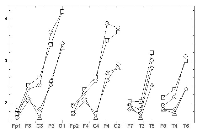
of three basic references. Fig.1 for chosen examinee presents the average
amplitudes Amean for three basic references in its ungrounded and grounded
states denoted below as Ch2, Bc, 2Nc and Ch2g, Bcg, 2Ncg. We can see the
obvious topographical differences between references and mutual displacement
of Amean. The comparison of fig.1A,B also shows the presence of some intraindividual
variability among two consecutive records.
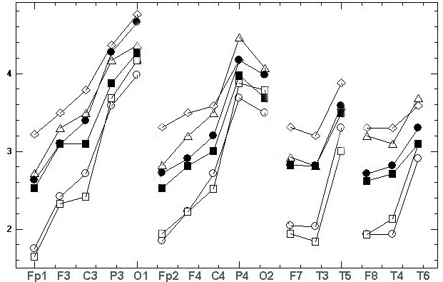
A
B
Fig. 1. Mean EEG spectral amplitudes
[mV] of alpha domain at 16 electrodes ordered
along sagittally meridians (horizontal axis). Six diagrams for chosen examinee
represent 6 records performed using three basic references in their ungrounded
state: at chin (Ch2), at back (Bc) and “united neck” (2Nc) and in their
grounded state (Ch2g, Bcg, 2Ncg) in two consecutive records (A, B). The
legends are on fig.1A.
Let us for each subject,
record and reference calculate M(Amean)-value by averaging of Amean over
the scalp. Fig.2 shows the changes of M(Amean) for three basic reference
electrodes, their two states (grounded/ungrounded), ten subjects and two
consecutive records for each subject. We can see that the data are characterized
by a strong interindividual variability. It also demonstrates (when comparing
two values for two consecutive records) the presence of intraindividual
variability, which is significantly lower in comparison with the interindividual
variability.
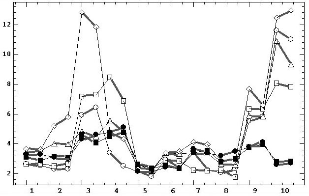
Fig. 2. Diagrams of mean spectral amplitudes
averaged over scalp [mV] in alpha domain for
ten subjects (horizontal axis) in six experiments using three basic reference
electrodes in their ungrounded and grounded states. For each subject, two
adjacent points on the diagrams, connected by bold lines, belong to two
consecutive records. The legends are similar to fig.1. Thin lines play
a supporting role for the connecting of the points of each of the six diagrams.
First, let us consider
the ratios between references in respect of their average tendencies. The
mean values and standard deviations of twenty M(Amean)-values calculated
for twenty records of each basic reference are: Bc=4.54±2.21, Bcg=5.88±3.67,
Ch2=4.1±2.87, Ch2g=4.42±2.5, 2Nc=3.4±0.87, 2Ncg=3.35±0.75. Thus, the greatest
average amplitude M(Amean) is observed for reference on back, then for
reference on chin and lowest one for “united neck” reference. The ratios
between these three references in grounded state are approximately double
that can be seen from statistics on their differences: Bcg-Ch2g=0.95±1.9,
Ch2g-2Ncg =0.88±2.55. Two-sample t-test does not find the differences between
Bcg and Ch2g, Ch2g and 2Ncg, Bc and Ch2, Ch2 and 2Nc at significance levels
p = 0.15, 0.07, 0.59, 0.31, t-values = 1.47, 1.85, 0.55, 1.03, DOF = 38,
22, 38, 22 (someone with Welch correction).
The statistics for
differences between grounded and ungrounded conditions: Bcg-Bc=1.33±2.38,
Ch2g-Ch2=0.32±1.93, 2Ncg-2Nc=-0.05±0.28 shows that increasing of averaged
EEG activation take its place for grounding state of references on back
and on chin. No significant differences between Bcg and Bc, Ch2g
and Ch2, 2Ncg and 2Nc were found at significance levels p = 0.17, 0.7,
0.8, t-values = 1.40, 0.39, 0.23, DOF = 31, 38, 38 (the first with Welch
correction).
The analysis of the
differences between grounded and ungrounded state of basic references requires
considering that the raw data are not simultaneously recorded, so the intraindividual
variability can affect the results of the comparison, and the extent of
this influence should be assessed in advance. The presence of two successive
records performed in each experiment helps to distinguish the correlations
determined by the intraindividual variability and by the influence of the
grounding factor (GF). Three above-described primary topographical indicators
Amean, DAmean1, DAmean2
are separately used as the raw data. The correlation between the presence/absence
of grounding was calculated for each parameter and ten subjects and for
two consecutive records reflecting the impact of intraindividual variability.
If the grounding
actually has a significant effect on the topography change, topograms for
grounded and ungrounded states would have greater differences than in the
case of natural intraindividual variability (appearing as a random and
less significant factor). Then, the correlations between the same primary
topographical indicators would be repeatedly weaker than in the case of
intraindividual variability. Therefore, the effect of GF can be detected
by pairwise comparing the mean values in the samples relating to GF and
intraindividual variability.
We explain the procedure
on the example of Amean values for grounded/ungrounded state. Pearson correlation
was calculated between Amean of 21 scalp derivations for each pair of Ch2-Ch2g,
Bc-Bcg 2Nc-2Ncg basic references records. Thus, the sample of 60 correlations
is formed, i.e. 3 basic references * 2 consecutive records * 10 subjects
= 60. This sample reflects GF. Similarly, the second sample of 60 correlations
between Amean values of the first and second consecutive records is formed,
i.e. 3 basic references * 2 grounded/ungrounded state * 10 subjects. The
second sample reflects intraindividual variability of Amean. For three
indicators Amean, DAmean1, DAmean2
we get three pairs of such samples.
Let us consider the
descriptive statistics (mean ± standard deviation) for the three pairs
of samples: 0.9 ± 0.12 and 0.92 ± 0.09 (correlations with Amean); 0.82±0.2
and 0.84±0.15 (DAmean1); 0.67±0.33 and 0.76±0.21
(DAmean2). The mean values of the correlations
related to GF, as expected, are slightly lower compared to intraindividual
variability (the difference of 2%, 2%, 14%, respectively) in all three
cases. However, t-test for correlations transformed by Fisher Z-normalization
Z(r)=0.5ln((1+r)/(1–r)) did not reveal significant differences between
means at significance levels р = 0.89, 0.67, and 0.98. Therefore, these
three indicators were not affected by GF beyond the effect of intraindividual
variability.
We can go the other
way. Our three pairs of samples represent two factors: 1-st factor with
two levels: GF - intraindividual variability, and 2-nd factor with three
levels: Amean, DAmean1, and DAmean2.
Sixty repeated values were measured for each factor level, but it is not
the third within-subjects factor because records in each pair of samples
are different. So we have the two-factors repeated measures model with
fixed-effects. This ANOVA got the results: 1-st factor effect: F(1,354)=0.292,
p=0.768; 2-nd factor effect: F(2,354)=12.67, p=0.00004; inter-factor effect:
F(2,354)=0.063, p=0.94. Thus, GF is not significant again.
These results are
further confirmed by cross correlations within the triad of the analyzed
samples related to Amean and ?Amean1, Amean and ?Amean2, ?Amean1 and ?Amean2.
These cross correlations affected by GF are 0.68, 0.63, 0.69, and effected
by intraindividual variability are 0.55, 0.31, 0.54. As we can see, the
former are repeatedly higher; i.e., GF correlations between the three pairs
of samples are more coordinated than those related to intraindividual variability.
Therefore, in this case, there is also no reducing effect of GF on the
correlations.
Conclusion.
Based on the results described above, grounded and ungrounded states of
reference electrodes can be considered equivalent in terms of preserving
the EEG topography.. This result in a certain degree reduces the relevance
of the problem to find or construct an infinitely remote neutral reference.
Indeed, why mathematically construct different virtual neutral references,
if the real neutral reference can be obtained under grounded electrode
on human body?
3.2. Topographic differences
between references
Based on the identified
equivalence, the records in this section were carried out with three conventional
ungrounded basic reference electrodes. Unlike the previous section, the
below comparisons were made within the same record of each subject arithmetically
transformed to different reference schemes. This allowed us to obtain quantitative
estimates of topographical differences caused by individual reference electrodes
without the influence of intra- and interindividual variability.
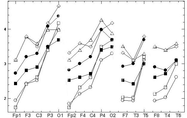
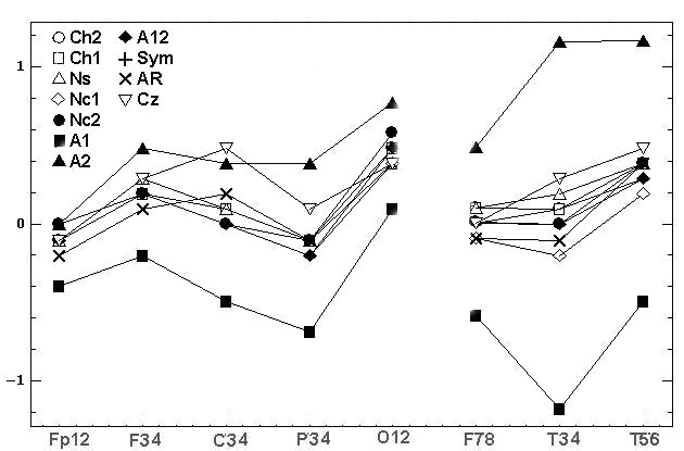
Fig.3 shows 11 diagrams
of mean spectral amplitudes of chosen subject and his record with basic
reference Ch2, this record was transformed to 11 reference schemes. On
fig 3 the topographical differences between some of the reference schemes
were evident. Moreover, we can see the EEG amplitude ratios of opposite
sign between electrodes F3 and C3, P3 and O1, Fp2 and F4, F4 and C4, P4
and O2, F7 and T3, F8 and T4 for different reference schemes. This situation
is very alarming because researchers using different reference schemes
can obtain results and make conclusions incomparable between themselves
and even contradictory in some cases
.
A
B
C
Fig. 3. The estimated indicators values [mV]
in alpha domain: A - average spectral amplitude Amean; B - differences
DAmean1
of Amean between couples of EEG derivations in saggital direction; C –
differences DAmean2 of Amean between symmetric
couples of derivations. Initial record was performed for chosen examinee
with basic reference at bottom of chin (Ch2), then it was mathematically
transformed to 11 reference schemes. Legends of references are on fig.3C:
bottom of chin (Ch2); top of chin (Ch1), nose (Ns), bottom of neck (Nc1),
top of neck (Nc2), A12, A1, A2, ipsilateral ears (Sym), averaged reference
(AR), vertex (Cz)
The final aim of our study is to find the
reliable classification of examined references according to their topographical
coherency was carried out using the following technique:
(1) Mi(rij) values were
transformed to uniform range by its ranking for better comparability.
(2) The mean rank of each reference scheme was calculated for each
subject.
(3) Using the resulting matrix of mean ranks, the K-means cluster
analysis of reference schemes in 10-dimentional space of 10 subjects with
Euclidian metric was conducted.
(4) The resulting classification is statistically verified by discriminant
analysis [17].
Table 1 shows the first step of this procedure
for chosen subject, i.e. averaged correlations Mi(rij),
their ranks and averaged ranks. Ranking is carried out by rows of table
top part, and these ranks (low part of table) are averaged for each reference
(through columns). Table 2 includes the averaged ranks of 10 subjects and
results of reference schemes classification.
Table 1. Results of topographical comparison of 13
references for chosen subject. At the upper part the averaged correlations
Mi(rij) (rows) for Amean, DAmean1,
DAmean2
estimates are presented for all references (columns). At the low part the
ranks of those correlations are calculated through each upper row followed
by mean rank of each reference.
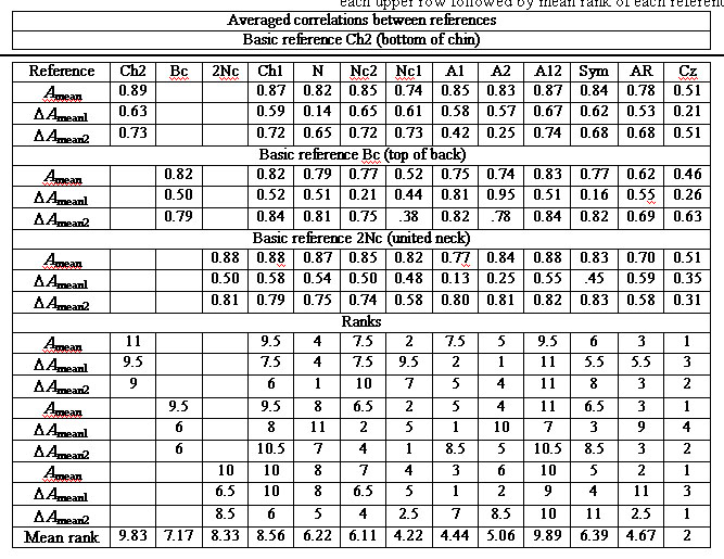
Table 2. Mean ranks of topographic coherency of 13
reference schemes (columns) and ten subjects (upper 10 rows) with their
clustering results and discriminant verification (lower four rows)
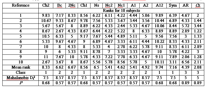
The clustering into
two, three, four, and five classes was tested. The only statistically significant
classification (p<0.0001 for the null hypothesis “the intercluster distance
is zero” or more popular “the classification is not valid”) includes the
three classes (cf. “Class” row in table 2). Number of class increases with
increasing of topographic incoherence of reference schemes. Two bottom
lines of the table show the Mahalanobis distance Di2 of each i-reference
scheme to its cluster center and the significance p of the null hypothesis
“Di2=0” meaning “the reference scheme belongs to this cluster.” All null
hypotheses are accepted at the highest significance levels p=0.57-0.89.
For relative estimation of references the table also includes their averaged
ranks (cf. “Mean rank” row).
Thus, the following
three classes of reference schemes were found:
(1) Reference electrodes
A12, Ch1, Ch2, and Sym (average ranks of 9.7, 8.6, 8.3, and 7.2) are characterized
by the highest similarity of their topography among themselves and in relation
to other references.
(2) Reference electrodes
2Nc, Bc, Ns, A1, Nc2, A2, and Nc1 (ranks 6.7, 6.6, 6.5, 5.4, 5.4, 4.9,
and 4.6) are characterized by less coherent topography.
(3) Reference electrodes
AR and Cz (ranks 4.4 and 2.1) are characterized by the least coherent topography.
3.3. Comparison with the standardized
reference
Now it is useful to compare
the above described results with the mathematical methods of designing
of a virtual neutral referents (see in Introduction). The best known and
most cited of these methods is REST [27, 34]. To demonstrate the inadequacy
of this method it is enough to take only a single example with the typical
EEG topography.
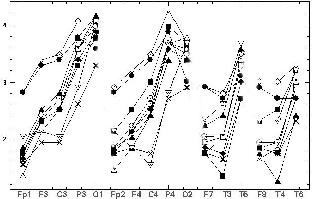
Let us take the two
consequential recordings of one subject (shown at fig.1) using the grounded
reference at the bottom of chin (Ch2g). Since these two records are made
without any time interval, then the general topographical relations should
be enough stable. On the other hand, the use of the grounded reference
is a guarantee of correct EEG amplitude values. Finally, this reference,
as it follows from table 2, has the highest topographic consistency with
other references, which further demonstrates the adequacy of obtained topographic
relationships. These two records were "standardized" according REST method
with subsequent calculation of Amean average amplitudes in the alpha domain,
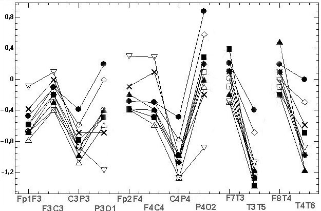
the comparative results are shown at fig.4.
а)
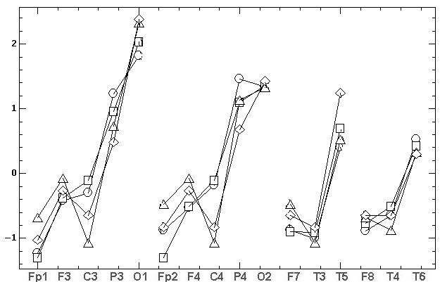
б)
Fig.4. The topographic relationships (similar
to fig.1) for two consecutive records, made by the grounded reference at
the bottom of the chin (Ch2g). The marks are: the circles and triangles
– the first and the second source records, the squares and diamonds – the
results of REST standardization. At fig. 4B the natural amplitudes of fig.
4A [mV] are Z-normalized for comparability.
As it can be seen
from fig. 4A the REST leads to the significant decrease of EEG amplitudes.
The average values of two source records are 2.67±0.83 and 2.69±0.73
compare to the REST values 2.18±0.49 and 2.19±0.52. In addition, REST brings
considerable topographical distortion, namely:
• the sharp decrease of C3 and C4 amplitudes
relative to all other electrodes;
• the significant decrease of P3 and P4 amplitudes
relative to O1 and O2; of T3 and T4 amplitudes relative to F7 and
F8;
• the significant increase of Fp1, Fp2, F3
and F4 amplitudes relative to P3, P4, O1 and O2; of T5 amplitude relative
to T6; of O1 amplitude relative to O2;
• the inversion of amplitude difference between
first and second records in Fp1, F7, F8, F3, F4, T6, O1, O2 electrodes;
• change the asymmetry sign: 1) in first record
between F3–F4, C3–C4, T5–T6 pairs of electrodes; 2) in second record between
Fp1–Fp2, F7–F8, F3–F4, C3–C4 pairs of electrodes.
Let us perform the
calculation of the absolute differences between the first and second records
for normalized date (fig. 4B). For the source records we receive smaller
difference 0.15±0.13 that differ 1.67 times from the results of REST standardization
0.25±0.18. One-sample Wilcoxon W-test (both samples belong to the same
sequence of derivations and the samples are not normally distributed according
chi-square test p=0.012) reveals the significant differences of these samples
p=0.013. Thus the differences between REST results significantly exceed
the intra-individual variability.
It should be also
noted that REST software contains a number of bags in its transformations
and processing, in import/export procedures, it is very poorly and fragmentary
documented, it supports only three schemes strictly fixed and very peculiar
sequence of 16, 64 and 128 EEG electrodes. So the use of this program is
only possible after a series of personal consultations with the authors.
These problems cause additional distrust of this method.
Thus, the REST method
brings the significant distortions in typical EEG topography provided using
the real neutral reference. Therefore, the advantages of REST method proclaimed
in numerous publications give raise to serious doubts.
4. Discussion
Among the many publications
on the subject, only small numbers of studies are focused on the comparison
of actual reference schemes used in research and clinical practice (it
is discussed in Ng and Raveendran, 2007; Alhaddad, 2012). Most studies
are concerned with general characteristics of the problem and discuss the
views of previous authors and present new mathematical methods for the
calculation of virtual reference electrodes that rather have theoretical
research value than the actual use and verification in practice. They propose
methods and compare them with other analogs and selected actual reference
electrodes, mostly with AR, or rarely A12 [10, 11, 20, 27, 32] using the
examples of simulation signals and selected EEG records.
The results are illustrated
by examples of EEG records, the amplitude spectra, power spectra, and topographic
maps, which in turn are compared and evaluated on the basis of visual inspection
with a purely qualitative verbal assessments and conclusions [2, 4, 10,
11, 21, 22, 29, 30]. Some studies implement quantitative assessment of
correlations, means, and signal/noise ratio and illustrate them with timeline
charts, scattering diagrams, and bar charts with standard errors [6, 34]
also discussed mainly with qualitative assessments. And only few papers
present the statistical analysis of hypotheses, pairwise comparisons by
Student’s t-test and ANOVA [8, 20, 27], which, however, do not relate to
differences of complex reference schemes but only their local aspects.
Thus, despite the 65-year discussion of the problem, no quantitative criteria
have been developed to compare and evaluate the benefits of using various
EEG reference electrodes.
In contrast, our
task was to assess the impact of existing reference electrodes used in
research and clinical practice on the EEG topography. For comparison of
the topographic proximity of reference schemes, we used three orthogonal
parameters and a new classification technique. On this basis, the studied
reference electrodes were divided into three classes according to their
proximity and differences in the topography of distribution of the mean
spectral amplitude on the scalp. The reliability of such a classification
is statistically valid. In this study, we also investigated for the first
time the effect of the grounded (electrically neutral) reference electrodes
in order to identify the advantages of their use.
Please note that
till now nobody came to the simple idea that if a reference electrode would
be directly connected with Earth ground, then we obtain the true zero potential
under this electrode on human body. If the scalp potentials are measured
relative to such reference then we get their true values relative to unchanged
zero potential. Indeed, previously, such measurements were impossible because
an amplifier was powered from the electric grid voltage of 220 volts. It
conflicts with the requirements of electrical safety of the subject. Newest
circuit design of amplifiers uses power via USB port of 5 volts located
in the electrically insulated notebook powered by its own direct current
battery. So, it is totally safe for the subject, and he can be directly
grounded during EEG recording.
Our introduction
shows that the efforts of many researchers have been focused on the search
for neutral reference that would ensure the recording of the true values
of EEG potentials, and thus attain the true or “ideal” topography of their
distribution over the scalp. We have created such neutral, remote from
the scalp references by their grounding. Then we found some usually used
ungrounded references providing topography closest to this “ideal”. Therefore,
we suppose that these references can be primarily recommended for use in
practice.
5. Conclusion
(1) We found no benefits
in using either grounded or ungrounded basic reference electrodes. These
conditions can be considered equivalent in terms of preserving the topography
of EEG potentials that in a certain degree reduces the relevance of the
tasks of searching and mathematical construction of an infinitely distant
neutral reference electrode.
(2) Reference electrodes
A1, Nc2, A2, Nc1, AR, and Cz (in descending ranks order) are characterized
by great topographic differences; thus, their use can lead to inconsistency
of the results and conclusions.
(3) The reference
electrodes with the most coordinated EEG topography include A12, Ch1, Ch2,
and Sym. Taking into account the first conclusion, we assumed that these
reference electrodes provide the most adequate EEG topography. Regarding
the most commonly used A12 scheme, the EEG correlations with proximal to
A1 and A2 electrodes T3 and T4 are quite strong: approximately 0.75–0.8.
However, the correlation with A1–A2 is substantially weaker, approximately
0.35–0.45, and approximately 0.17–0.2 for the T3 and T4. Therefore, the
combining of the ear electrodes does not lead to any significant distortions
in the “true” topography of EEG potentials.
.
References
[1] Adrian E. D., Matthews B. H.
(1934) The Berger rhythm: potential changes from the occipital lobes in
man. Brain. 57:355–385.
[2] Alhaddad M. J. (2012) Common
Average Reference (CAR) Improves P300 Speller. Int J Eng Technol. 2(3):451–463.
[3] Berger H. (1929) Uber das
Elektroenkephalogramm des Menschen. Archiv fur Psychiatrie und Nervenkrankheiten.
87:527–570.
[4] Carvalhaes C. G., Suppes
P. (2011) A spline framework for estimating the EEG surface Laplacian using
the Euclidean metric. Neural Comput. 23(11):2974–3000.
[5] Desmedt J.E., Chalklin V.,
Tomberg C. (1990) Emulation of somatosensory evoked potential (SEP) components
with the 3-shell head model and the problem of ‘ghost’ potential fields’
when using an average reference in brain mapping. Electroenceph Clin Neurophysiol
77(4):243–258.
[6] Essl M., Rappelsberger P.
(1998) EEG coherence and reference signals: experimental results and mathematical
explanations. Med Biol Eng Comput. 36(4):399–406.
[7] Fingelkurts A., Fingelkurts
A., Krause C., Kaplan A., Borisov S., Sams M. (2003) Structural (operational)
synchrony of EEG alpha activity during an auditory memory task. Neuroimage.
20(1):529–542.
[8] Hagemann D., Naumann E.,
Thayer J.F. (2001) The quest for the EEG reference revisited: A glance
from brain asymmetry research. Psychophysiol. 38(5):847–857.
[9] Hjorth B. (1975) An on-line
transformation of EEG scalp potentials into orthogonal source derivations.
Electroencephal. and Clin Neurophysiol. 39(5):526–530.
[10] Hu S., Cao Y., Chen S.,
Kong W., Zhang J., Li X., Zhang Y. (2012) Independence Verification for
Reference Signal under Neck of Human Body in EEG Recordings. Proc 31-th
Chinese Control Conf. Hefei. 4038-4042.
[11] Hu S., Cao Y., Chen S.,
Zhang J., Kong W., Yang K., et al. (2012) A comparative study of two reference
estimation methods in EEG recording. Proc Brain Inspir Cogn Syst. 321–328.
[12] Geselowitz D. B. (1998)
The zero of potential. IEEE Eng Med Biol Mag. 17(1):128–132,
[13] James C. J., Whesse C. (2005)
Independent component analysis for biomedical signals. Physiol Meas. 26:R15–39.
[15] Jasper H. H. (1958) The
ten-twenty electrode system of the International Federation. Electroencephal
Clin Neurophysiol. 10:371–375.
[16] Kayser J., Tenke C. E. (2010)
In search of the Rosetta Stone for scalp EEG: Converging on reference-free
techniques. Clin Neurophysiol. 121(12):1973–1975.
[17] Klecka W. R. (1980).Discriminant
Analysis. SAGE Publications. 72 pp.
[18] Kulaichev A. P. (2011) The
method of correlation analysis of EEG synchronism and its possibilities.
Zh Vyssh Nerv Deiat Im I P Pavlova. 61(4):1–14.
[19] Kulaichev A. P., Gorbachevskaya
N.L. (2013) Differentiation of Norm and Disorders of Schizophrenic Spectrum
by Analysis of EEG Correlation Synchrony. J Exp Integr Med. 3(4):267–278.
[20] Lepage K. Q., Kramer M.
A., Chu C. J. (2014) A statistically robust EEG re-referencing procedure
to mitigate reference effect. J Neurosci Methods. 235(30):101–116.
[21] Madhu N., Ranta R., Maillard
L., Koessler L. A. (2012) Unified treatment of the reference estimation
problem in depth EEG recordings. Med Biol Eng Comput: 50(10):1003–1015
[22] Marzett L., Nolte G., Perrucci
M. G., Romani G. L., Del Gratta C. (2007) The use of standardized infinity
reference in EEG coherency studies. Neuroimage. 36(1):48–63
[23] Ng S. C., Raveendran P.
(2007) Comparison of different Montages on to EEG classification. Biomed
06, IFMBE Proceedings 15, 365–368.
[24] Nunez P. L. (1981) Electric
fields of the brain: the neurophysics of EEG. Oxford Univ. Press. NY. 640
pp.
[25] Pascual-Marqui R. D., Lehmann
D. (1993) Topographic maps, source localization inference, and the reference
electrode. Electroenceph Clin Neurophysiol, 88(6):532–536.
[26] Perrin F., Pernier J., Bertrand
O., Echallier J. F. (1989) Spherical splines for scalp potential and current
density mapping. Electroenceph Clin Neurophysiol, 72(2):184–187.
[27] Qin Y., Xu P., Yao D. (2010)
A comparative study of different references for EEG default mode network:
the use of the infinity reference. Clin. Neurophysiol. 121(12):1981–1991.
[28] Schiff S. J. (2006) Dangerous
Phase, Neuroinformatics. 3(4): 315–318.
[29] Stephenson W. A., Gibbs
F. A. (1951) A balanced non-cephalic reference electrode. EEG Clin. Neurophysiol.
3:237–240.
[30] Tenke C. E., Kayser J. (2005)
Reference-free quantification of EEG spectra: Combining current source
density (CSD) and frequency principal components analysis (fPCA). Clin
Neurophysiol. 116(12):2826–2846.
[31] Teplan M. (2002) Fundamentals
of EEG mesurement. Meas Sci Rev. v.2, sect.2: 1–11.
[32] Wang B., Wang X., Ikeda
A., Nagamin T., Shibasaki H., Nakamuraea M. (2014) Automatic reference
selection for quantitative EEG interpretation: Identification of diffuse/localised
activity and the active ear lobe reference, iterative detection of the
distribution of EEG rhythms. Med Eng Phys. 36(1):88– 95.
[33] Wolpaw J. R., Wood C. C.
(1982) Scalp distribution of human auditory evoked potentials. Evaluation
of reference electrode sites. Electroenceph Clin Neurophysiol. 54(1):15–24.
[34] Yao (2001) A method to standardize
a reference of scalp EEG recordings to a point at infinity. Physiol Meas.
22(4):693–711.